Introduction to Data Pre-processing Techniques

Data pre-processing, also known as data cleaning or data wrangling, is a crucial step in data analysis. It involves transforming raw data into a format suitable for analysis. Here are the key topics covered in data pre-processing:

Identifying and Handling Missing Values

• Definition: Missing values occur when data entries are left empty.

• Techniques:
  • Removing or imputing missing values.

Standardizing Data Formats

• Issue: Data from different sources may be in various formats, units, or conventions.

• Solution: Use methods to convert and standardize data formats.

Data Normalization

• Purpose: Bring all numerical data into a similar range for meaningful comparison.

• Techniques: Centering and scaling data values.

Data Binning

• Purpose: Create larger categories from numerical values for easier comparison between groups.

• Technique: Dividing data into bins.

Handling Categorical Variables

• Issue: Categorical values need to be converted to numerical values for statistical modeling.

• Solution: Label encoding and one-hot encoding.

Manipulating Data Frames in Python

In Python, we usually perform operations along columns. Each row represents a sample (e.g., a different used car in the database). Here’s a quick overview of basic data manipulation:

• Accessing Columns: Columns can be accessed using their names. For example, df['symboling'] or df['body_style'].

• Pandas Series: Each column is a Pandas Series, a one-dimensional array-like object.

• Example Operation: Adding a value to each entry in a column.

  df['symboling'] = df['symboling'] + 1

These techniques ensure your data is clean, standardized, and ready for meaningful analysis and modeling.

1. Handling Missing Values in Data Pre-processing

Missing values are a common issue in datasets and occur when no data value is stored for a feature in a particular observation. These can appear as question marks, N/A, zeros, or blank cells. Effective handling of missing values is essential for accurate data analysis. Here are some strategies and techniques to deal with missing values:

Identification of Missing Values

• Common Representations: NaN, ?, N/A, 0, or blank cells.

• Example: The normalized losses feature has missing values represented as NaN.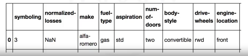

  

Strategies to Handle Missing Values

1. Recollection:
   • Check if the original data collectors can provide the missing values.

2. Removing Data:
   • Dropping Entries: Remove the entire row or column with missing values.
     • Suitable when only a few observations have missing values.
     • Example: If the price column has missing values and it's the target variable, drop the rows with missing prices.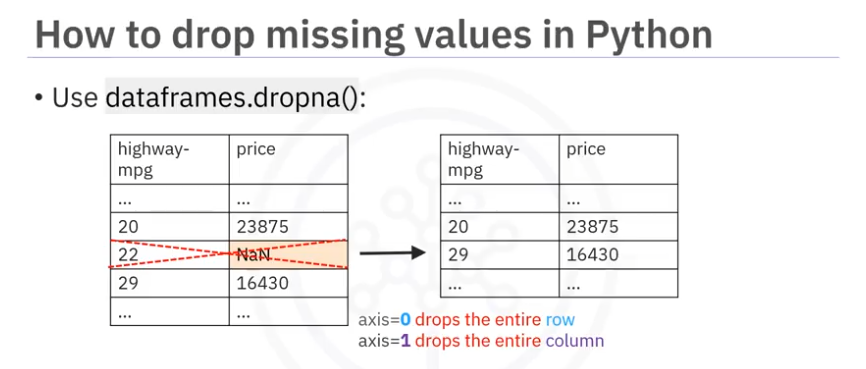

       

   • Pandas Method:

     df.dropna(axis=0, inplace=True)  # Drop rows with missing values
     df.dropna(axis=1, inplace=True)  # Drop columns with missing values

3. Replacing Data:
   • Mean/Median/Mode:
     • Replace missing values with the mean (for numerical data), median, or mode (for categorical data).
     • Example: Replace missing normalized losses with the mean of the column.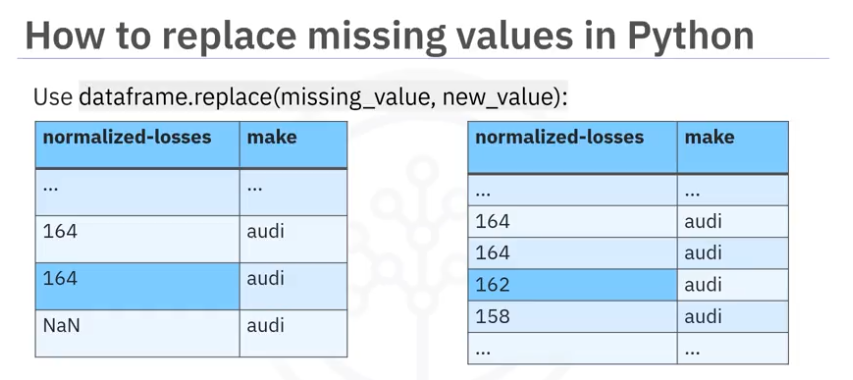

       

     • Pandas Method:

       mean_value = df['normalized_losses'].mean()
       df['normalized_losses'].replace(np.nan, mean_value, inplace=True)

   • Other Techniques:
     • Use group-specific averages or other statistical methods to impute missing values.
     • Example: Replace missing values based on the average within a subgroup of data.

4. Leaving Missing Data:
   • In some cases, it might be beneficial to retain missing values for specific analysis needs.

Practical Implementation in Python

1. Dropping Missing Values:
   • Drop rows with missing values in the price column:

     df.dropna(subset=['price'], axis=0, inplace=True)

2. Replacing Missing Values:
   • Calculate the mean of a column and replace NaNs:

     mean_value = df['normalized_losses'].mean()
     df['normalized_losses'].replace(np.nan, mean_value, inplace=True)

Conclusion

Handling missing values effectively is crucial for ensuring the accuracy and reliability of data analysis. The methods to handle missing values can vary based on the nature of the data and the analysis requirements. Using techniques like removing, replacing, or even retaining missing values with the right approach can significantly improve the quality of your data and the insights derived from it.

2. Handling Data with Different Formats, Units, and Conventions

Data collected from various sources often comes in different formats, units, and conventions. Data formatting is essential for ensuring consistency and facilitating meaningful comparisons. Let's explore how to address these issues using Pandas.

Importance of Data Formatting

• Consistency: Ensures that data is standardized for analysis.

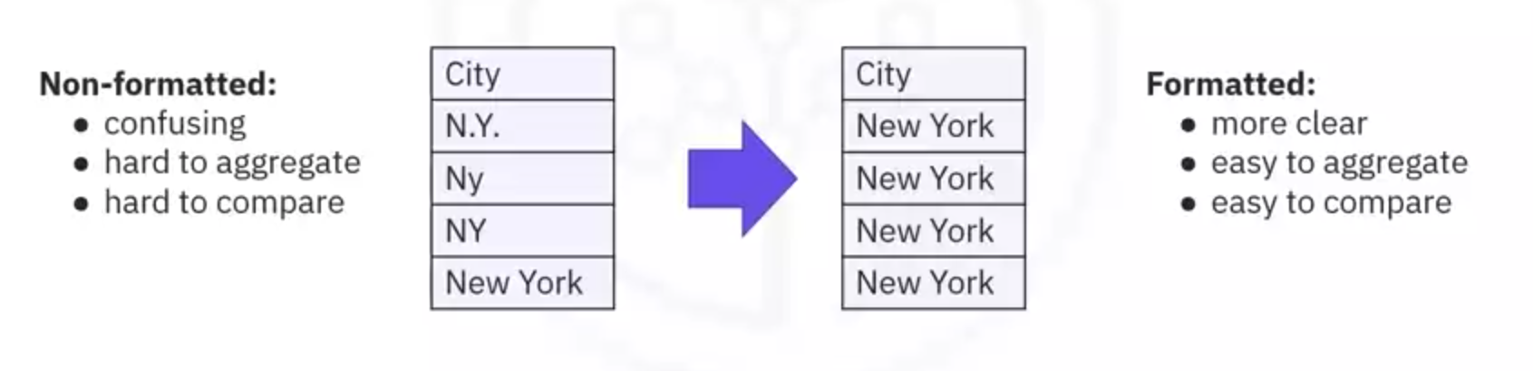
• Clarity: Makes data easily understandable.

• Examples: Representing "New York City" consistently as "NY" or converting measurement units for uniformity.

  

Common Issues and Solutions

1. Inconsistent Naming Conventions:
   • Example: Different representations of "New York City" such as "N.Y.", "Ny", "NY", "New York".
   • Solution: Standardize these entries to a single format for analysis.
   • Pandas Method:

     df['city'] = df['city'].replace({'N.Y.': 'NY', 'Ny': 'NY', 'New York': 'NY'})

2. Different Measurement Units:
   • Example: Converting miles per gallon (mpg) to liters per 100 kilometers (L/100km).
     • Conversion Formula: 235 / mpg
   • Implementation in Python:

     df['city-mpg'] = 235 / df['city-mpg']
     df.rename(columns={'city-mpg': 'city-L/100km'}, inplace=True))

3. Incorrect Data Types:
   • Example: A numeric column imported as a string (object) type.
   • Identifying Data Types: Use dataframe.dtypes() to check data types.
   • Converting Data Types: Use dataframe.astype() to change data types.
   • Implementation in Python:

     df['price'] = df['price'].astype('int')

Practical Implementation

1. Standardizing Entries:
   • Scenario: Different representations of "New York City".
   • Code Example:

     df['city'] = df['city'].replace({'N.Y.': 'NY', 'Ny': 'NY', 'New York': 'NY'})

2. Converting Units:
   • Scenario: Convert city-mpg to city-L/100km.
   • Code Example:

     df['city-mpg'] = 235 / df['city-mpg']
     df.rename(columns={'city-mpg': 'city-L/100km'}, inplace=True))

3. Fixing Data Types:
   • Scenario: Convert the price column from string to integer.
   • Code Example:

     df['price'] = df['price'].astype('int')

Conclusion

Data formatting is a crucial step in data pre-processing, ensuring consistency and accuracy in data analysis. Using Pandas, you can standardize naming conventions, convert measurement units, and correct data types efficiently. These practices help in preparing the data for more meaningful and accurate analysis.

By addressing these common data issues, you can enhance the quality and reliability of your datasets, leading to better insights and decisions.

3. Data Normalization

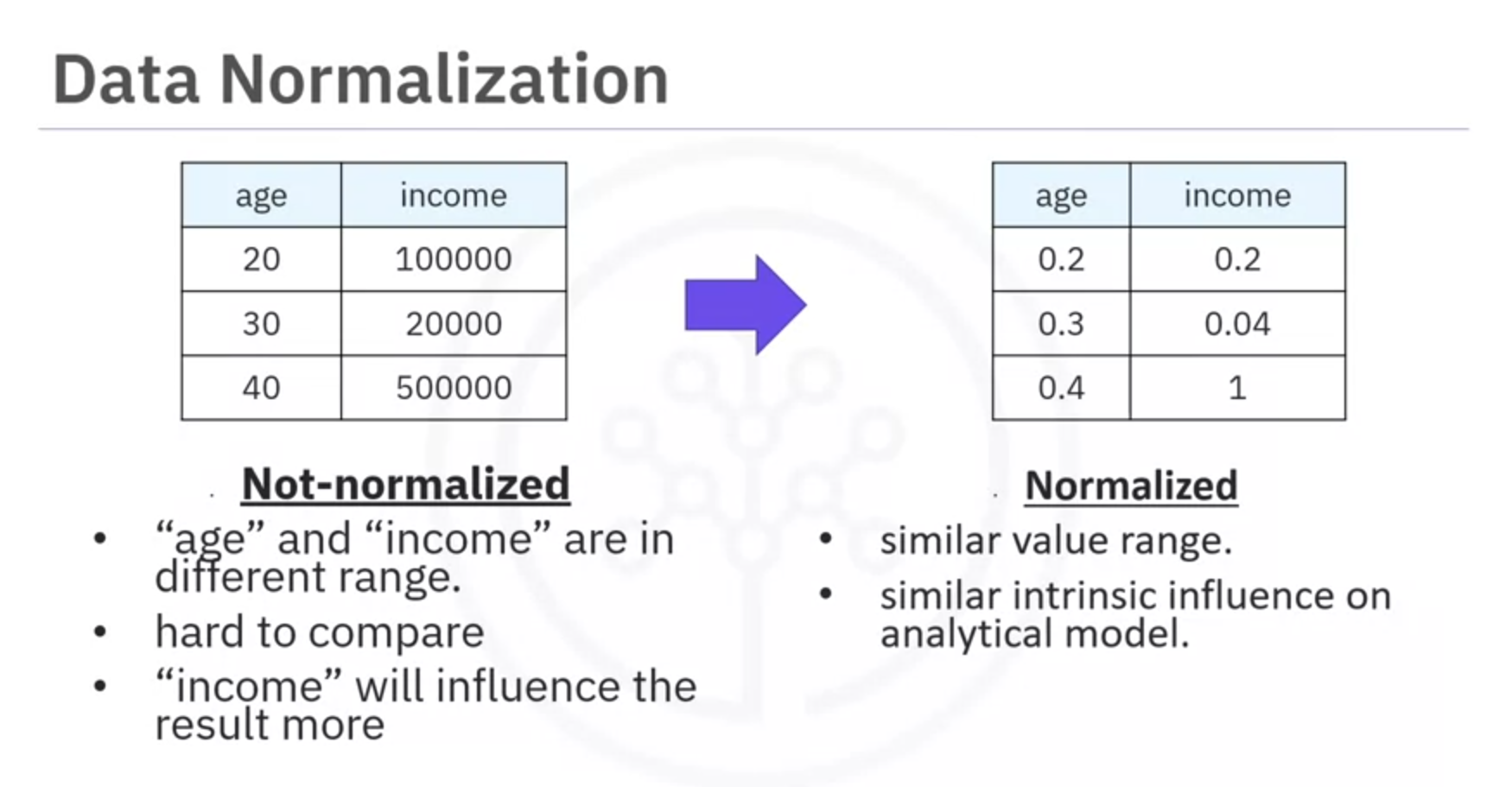
Data normalization is an essential preprocessing technique used to standardize the range of independent variables or features of data. This ensures that each feature contributes equally to the analysis and is crucial for computational efficiency and fair comparison between variables.

Why Normalize Data?

1. Consistency in Range:
   • Features like length, width, and height might have different ranges (e.g., length: 150-250, width/height: 50-100).
   • Normalizing ensures consistent ranges, facilitating easier statistical analysis.

2. Fair Comparison:
   • Different features might have varying impacts due to their range differences (e.g., age: 0-100, income: 0-20,000).
   • Normalization ensures each feature has an equal influence on the model.

3. Computational Efficiency:
   • Prevents features with larger ranges from dominating the model (e.g., in linear regression, larger value ranges might bias the model).

Methods of Normalization

1. Simple Feature Scaling:
   • Formula:

   $$x_{new} = \frac{x_{old}}{x_{max}}$$

   • Range: 0 to 1
   • Example in Python:

     df['length'] = df['length'] / df['length'].max()

     

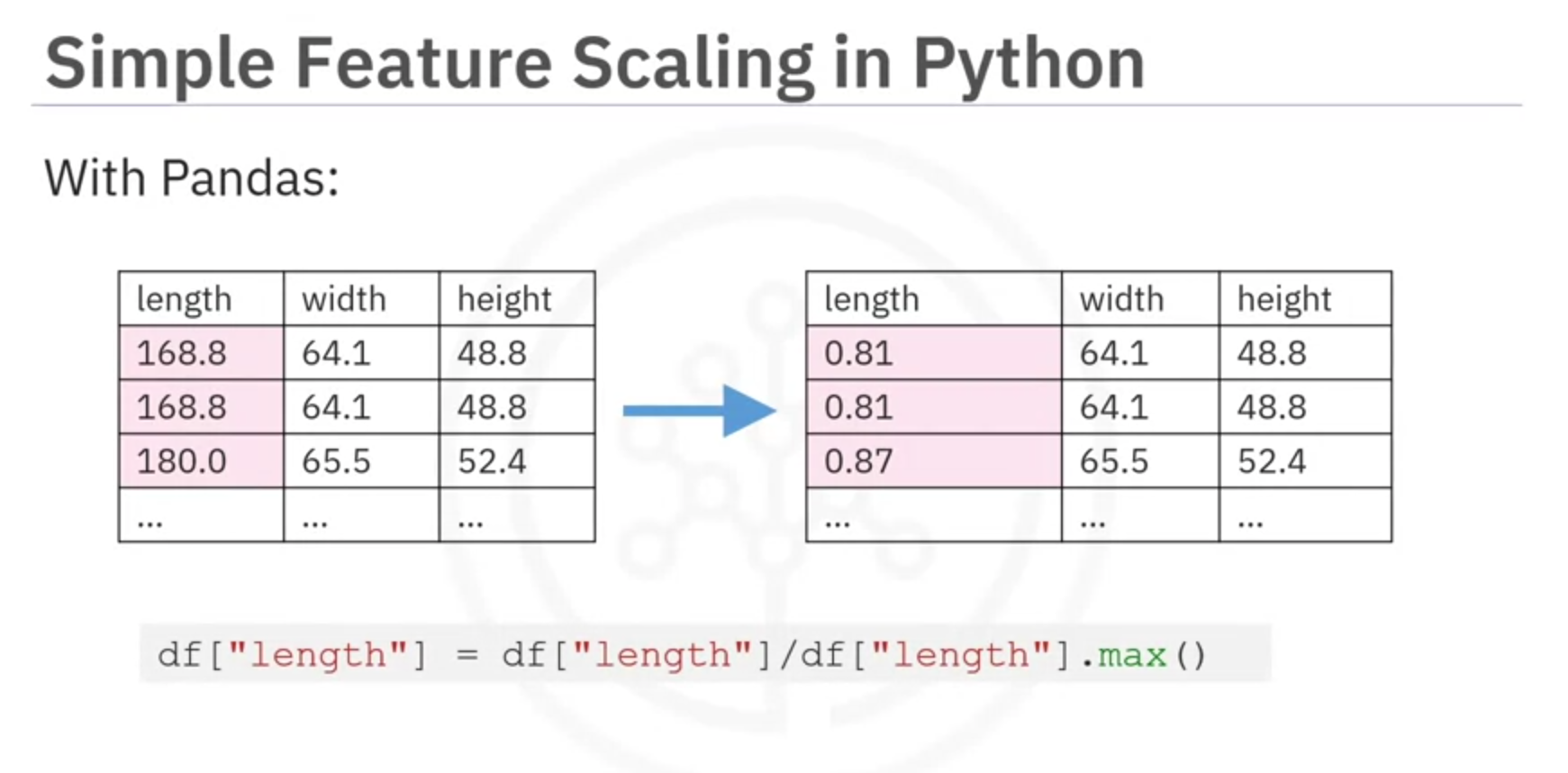
2. Min-Max Scaling:
   • Formula:

   $$x_{new} = \frac{x_{old} - x_{min}}{x_{max} - x_{min}}$$

   • Range: 0 to 1
   • Example in Python:

     df['length'] = (df['length'] - df['length'].min()) / 
     							 (df['length'].max() - df['length'].min())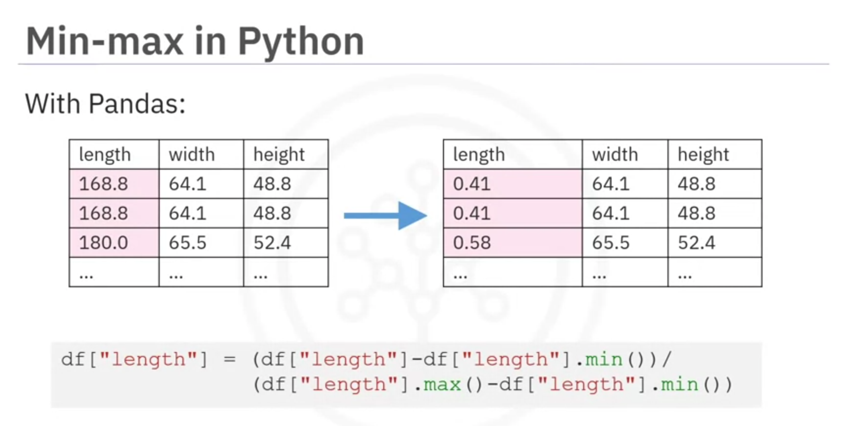

     

3. Z-Score (Standard Score) Normalization:
   • Formula:

   $$x_{new} = \frac{x_{old} - \mu}{\sigma}$$

   • Range: Typically -3 to +3
   • Example in Python:

     df['length'] = (df['length'] - df['length'].mean()) / df['length'].std()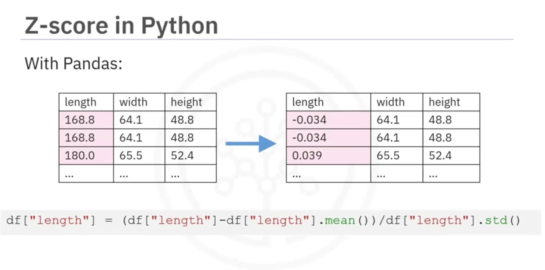

     

Example Implementation in Python

Given a dataset containing a feature length:

1. Simple Feature Scaling:

   df['length'] = df['length'] / df['length'].max()

2. Min-Max Scaling:

   df['length'] = (df['length'] - df['length'].min() /
   				       (df['length'].max() - df['length'].min())

3. Z-Score Normalization:

   df['length'] = (df['length'] - df['length'].mean()) / df['length'].std()

Conclusion

Normalization is a crucial step in preparing your data for analysis, ensuring all features contribute equally and improving the performance of your models.

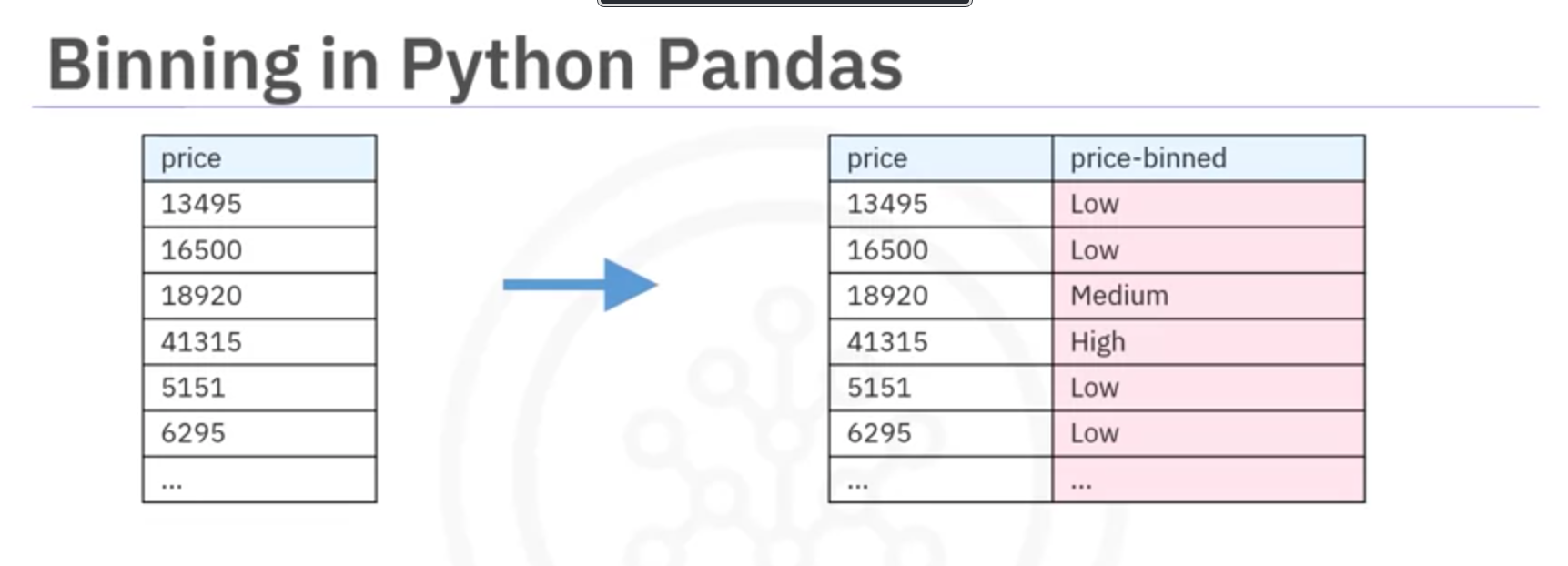
4. Data Binning

Binning is a data preprocessing technique where numerical values are grouped into bins or categories. This method can enhance the accuracy of predictive models and provide a better understanding of data distribution.

Why Bin Data?

1. Improves Model Accuracy: Grouping values can sometimes enhance the performance of predictive models.

2. Simplifies Analysis: Reducing the number of unique values can make data analysis more manageable and insightful.

Example:

• Age Binning: Grouping ages into bins like 0-5, 6-10, 11-15, etc.

• Price Binning: Categorizing car prices into low, medium, and high.

Application on Car Price Data:

• Range: The price ranges from $5,188 to $45,400 with 201 unique values.

• Binning: We categorize prices into three bins: low price, medium price, and high price.

Steps to Implement Binning in Python:

1. Determine Bin Dividers:
   • Use NumPy's linspace function to create equally spaced bin dividers.

   import numpy as np
   bins = np.linspace(min(df['price']), max(df['price']), 4)

2. Create Bin Labels:
   • Define the names of the bins.

   group_names = ['Low', 'Medium', 'High']

3. Apply Binning:
   • Use Pandas' cut function to bin the data.

   df['price_binned'] = pd.cut(df['price'],bins,labels=group_names,include_lowest=True)

4. Visualize Binned Data:
   • Use histograms to visualize the distribution of the binned data.

   import matplotlib.pyplot as plt
   plt.hist(df['price_binned'], bins=3, edgecolor='k')
   plt.xlabel('Price Bins')
   plt.ylabel('Number of Cars')
   plt.title('Histogram of Binned Car Prices')
   plt.show()

Example Code:

import numpy as np
import pandas as pd
import matplotlib.pyplot as plt

# Sample data
df = pd.DataFrame({'price': [5000, 10000, 15000, 20000, 25000, 30000, 35000, 40000, 45000]})

# Binning
bins = np.linspace(min(df['price']), max(df['price']), 4)
group_names = ['Low', 'Medium', 'High']
df['price_binned'] = pd.cut(df['price'], bins, labels=group_names, include_lowest=True)

# Visualization
plt.hist(df['price_binned'], bins=3, edgecolor='k')
plt.xlabel('Price Bins')
plt.ylabel('Number of Cars')
plt.title('Histogram of Binned Car Prices')
plt.show()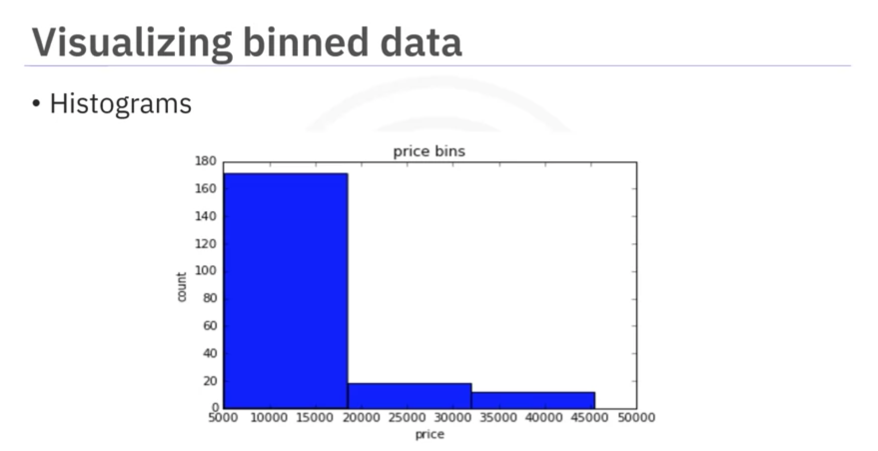

Conclusion

Binning is a powerful technique for simplifying data analysis and improving model performance. By categorizing continuous variables into discrete bins, we can gain clearer insights and more effectively leverage statistical methods.

5. Transforming Categorical Variables into Quantitative Variables

In data preprocessing, it's essential to convert categorical variables into a numeric format that statistical models can process. This process is often referred to as one-hot encoding.

Why Transform Categorical Variables?

• Statistical Models Requirement: Most models require numerical input.

• Improved Analysis: Converting strings to numbers allows for better analysis and model training.

Example: Fuel Type in Car Dataset

• Categorical Variable: The fuel type feature has values like "gas" and "diesel".

• Goal: Convert "gas" and "diesel" into numerical values for model training.

One-Hot Encoding

One-hot encoding involves creating new binary columns (features) for each unique category in the original feature. Each row is marked with a 1 or 0, indicating the presence or absence of the category.

Steps:

1. Identify Unique Categories: For the fuel type feature, identify unique values like "gas" and "diesel".

2. Create Binary Columns: Create new columns for each unique category.

3. Assign Binary Values: Set the value to 1 if the category is present, otherwise 0.

Example:

• Original Data:
  • Car A: gas
  • Car B: diesel
  • Car C: gas

• One-Hot Encoded Data:
  • Car A: gas = 1, diesel = 0
  • Car B: gas = 0, diesel = 1
  • Car C: gas = 1, diesel = 0

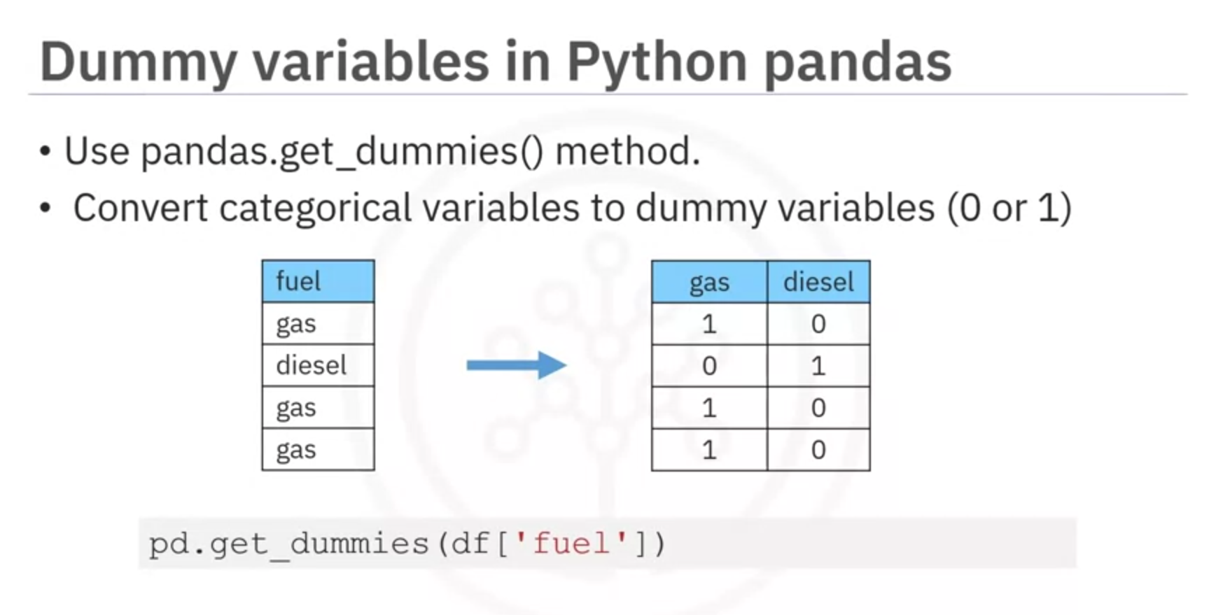
Implementing One-Hot Encoding in Python

Use the pd.get_dummies method from the Pandas library to perform one-hot encoding.

Example Code:

import pandas as pd

# Sample data
df = pd.DataFrame({'fuel': ['gas', 'diesel', 'gas']})

# One-hot encoding
dummy_variable = pd.get_dummies(df['fuel'])

# Combine with original dataframe
df = pd.concat([df, dummy_variable], axis=1)

print(df)

Output:

     fuel  diesel  gas
0     gas       0    1
1  diesel       1    0
2     gas       0    1

Indicator Variable

What is an indicator variable?
An indicator variable (or dummy variable) is a numerical variable used to label categories. They are called 'dummies' because the numbers themselves don't have inherent meaning.

Why use indicator variables?
You use indicator variables so you can use categorical variables for regression analysis in later modules.

Example

The column "fuel-type" has two unique values: "gas" or "diesel". Regression doesn't understand words, only numbers. To use this attribute in regression analysis, you can convert "fuel-type" to indicator variables.

Use the Pandas method 'get_dummies' to assign numerical values to different categories of fuel type.

Conclusion

Converting categorical variables into quantitative variables is crucial for statistical analysis and model training. One-hot encoding is a simple yet effective method to achieve this transformation, allowing categorical data to be used in numerical computations.

Cheat Sheet: Data Wrangling

Replace missing data with frequency

Replace missing values with the mode (most frequent value) of the column.

MostFrequentEntry = df['attribute_name'].value_counts().idxmax()
df['attribute_name'].replace(np.nan, MostFrequentEntry, inplace=True)

Replace missing data with mean

Replace missing values with the mean of the column.

AverageValue = df['attribute_name'].astype(data_type).mean(axis=0)
df['attribute_name'].replace(np.nan, AverageValue, inplace=True)

Fix the data types

Convert columns to the specified data type (e.g., int, float, str).

df[['attribute1_name', 'attribute2_name', ...]] = df[['attribute1_name', 'attribute2_name', ...]].astype('data_type')

Data Normalization

Normalize values in a column between 0 and 1.

df['attribute_name'] = df['attribute_name'] / df['attribute_name'].max()

Binning

Group data into bins for better analysis and visualization.

bins = np.linspace(min(df['attribute_name']), max(df['attribute_name']), n)
GroupNames = ['Group1', 'Group2', 'Group3', ...]
df['binned_attribute_name'] = pd.cut(df['attribute_name'], bins, labels=GroupNames, include_lowest=True)

Change column name

Rename a column in the dataframe.

df.rename(columns={'old_name': 'new_name'}, inplace=True)

Indicator Variables

Create dummy variables for categorical data.

dummy_variable = pd.get_dummies(df['attribute_name'])
df = pd.concat([df, dummy_variable], axis=1)