Module 4: Model Development

Introduction to Model Development

This module delves into the process of model development, focusing on predictive modeling using datasets. It covers various regression techniques, model evaluation methods, and the importance of accurate data in making predictions.

Key Concepts

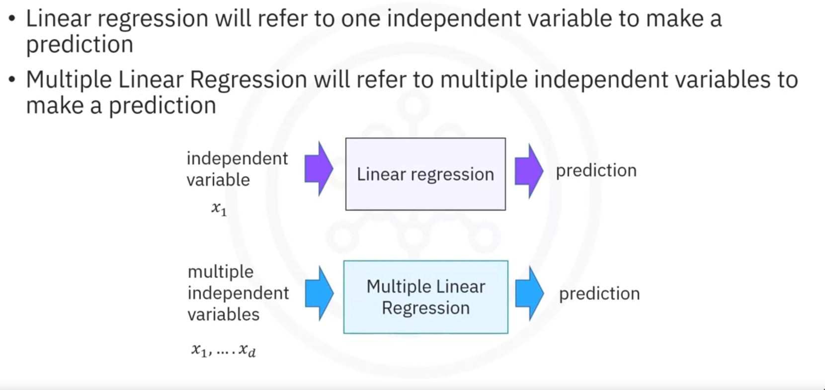
1. Simple and Multiple Linear Regression:

Use linear regression to predict outcomes based on one or more independent variables.

2. Model Evaluation Using Visualization:

Visually assess the performance of models.

3. Polynomial Regression and Pipelines:

Employ polynomial regression to capture non-linear relationships and implement pipelines for streamlined model building.

4. R-squared and Mean Squared Error (MSE):

Evaluate model performance using metrics such as R-squared and MSE to determine prediction accuracy.

5. Prediction and Decision Making:

Utilize models to make informed predictions and decisions based on the data.

Importance of Data

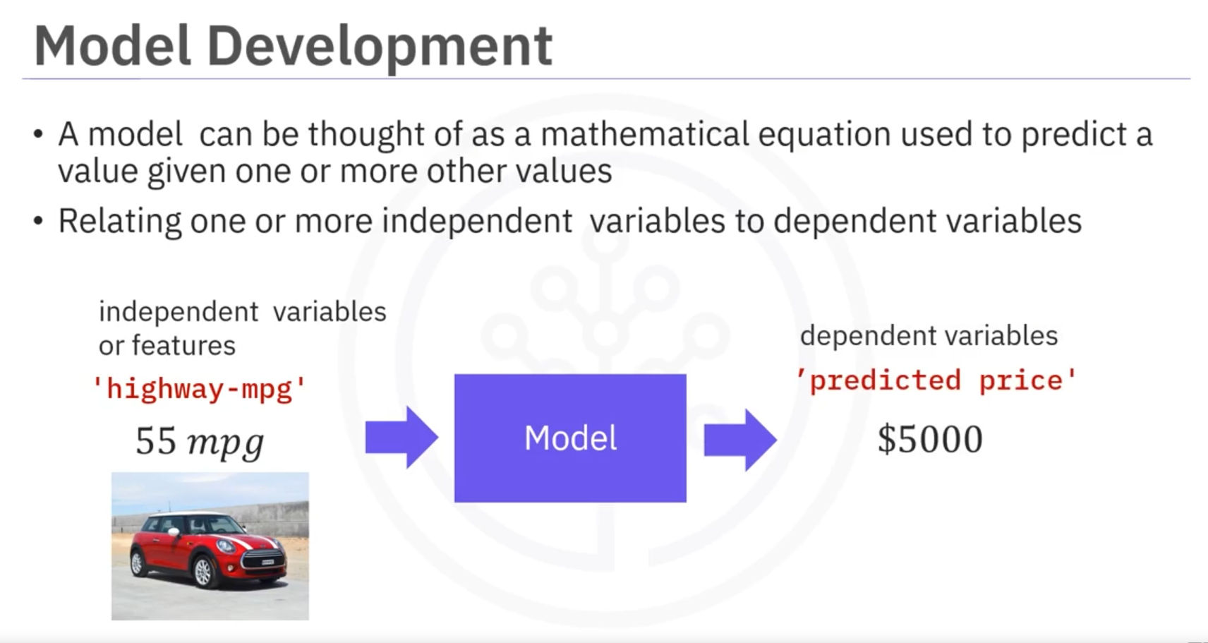
A model, or estimator, is essentially a mathematical equation that predicts a value based on one or more other values. It relates one or more independent variables (features) to dependent variables (outcomes). The accuracy of the model often improves with the relevance and quantity of data. Including multiple independent variables can lead to more precise predictions.

For instance, consider a scenario where predicting an outcome is based on several features. If the model's independent variables do not include a crucial feature, predictions may be inaccurate. Therefore, gathering more relevant data and exploring different types of models is cru1cial for robust model development.

1. Simple and Multiple Linear Regression

Linear Regression

Linear regression predicts a target value using one or more independent variables.

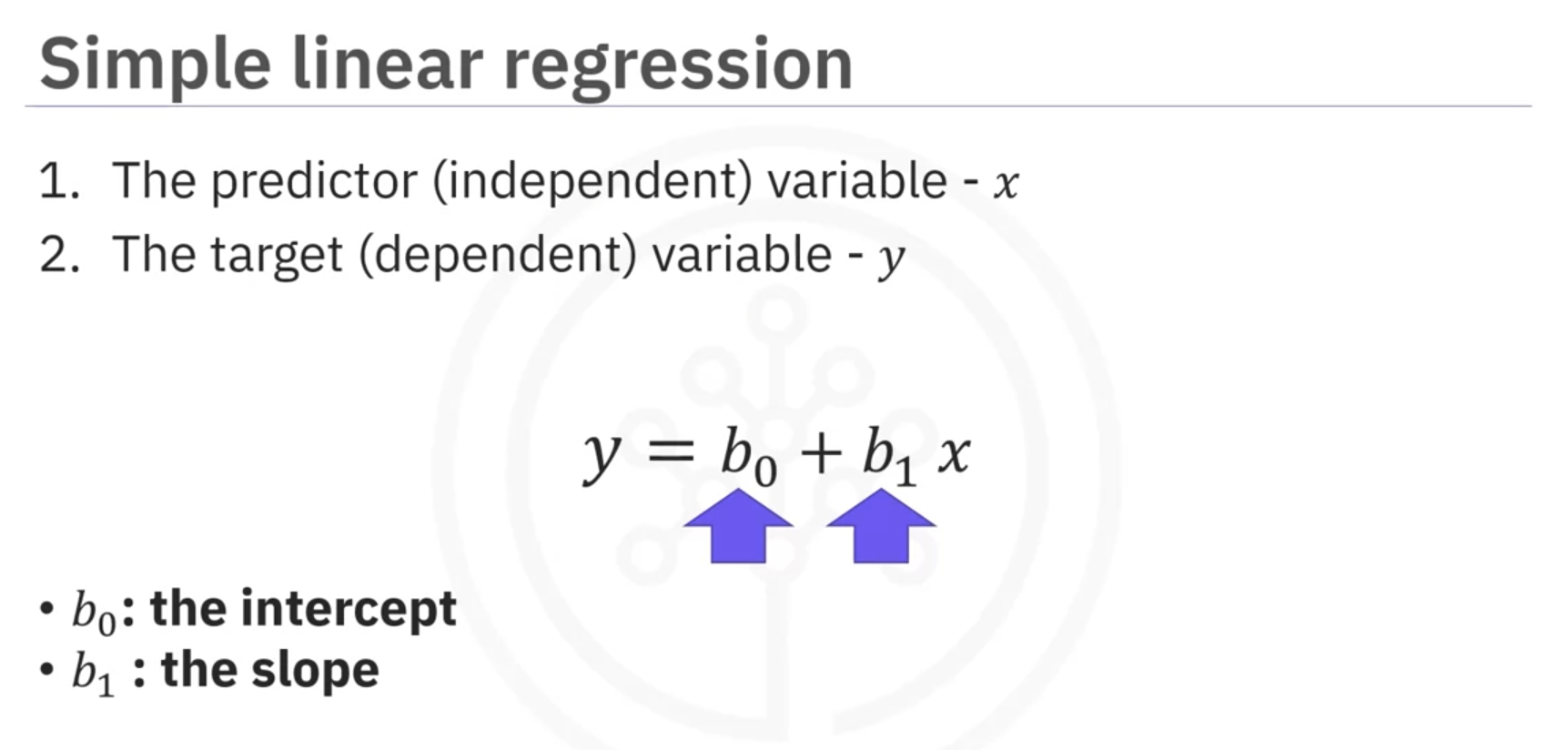
1.1 Simple Linear Regression (SLR)

SLR examines the relationship between two variables:

Predictor (independent variable $x$ )

Target (dependent variable $y$ )

The relationship is defined as:

$y = b_0 + b_1 x$

$b_0$ : Intercept

$b_1$ : Slope

Prediction Step

If highway miles per gallon is 20, a linear model might predict the car price as $22,000, assuming a linear relationship.

Training the Model

Data points are stored in data frames or NumPy arrays. The predictor values ( $x$ ) and target values ( $y$ ) are stored separately. The model is trained using these data points to determine the parameters $b_0$ and .

Handling Uncertainty

Factors like car make and age influence car prices. Uncertainty in the model is addressed by adding a small random value (noise) to the line. The noise is usually a small positive or negative value.

Python Implementation

from sklearn.linear_model import LinearRegression

# Create a linear regression object
lm = LinearRegression()

# Define predictor (x) and target (y) variables
x = ...
y = ...

# Fit the model
lm.fit(x, y)

# Make predictions
predicted_values = lm.predict(x)

# Model parameters
intercept = lm.intercept_
slope = lm.coef_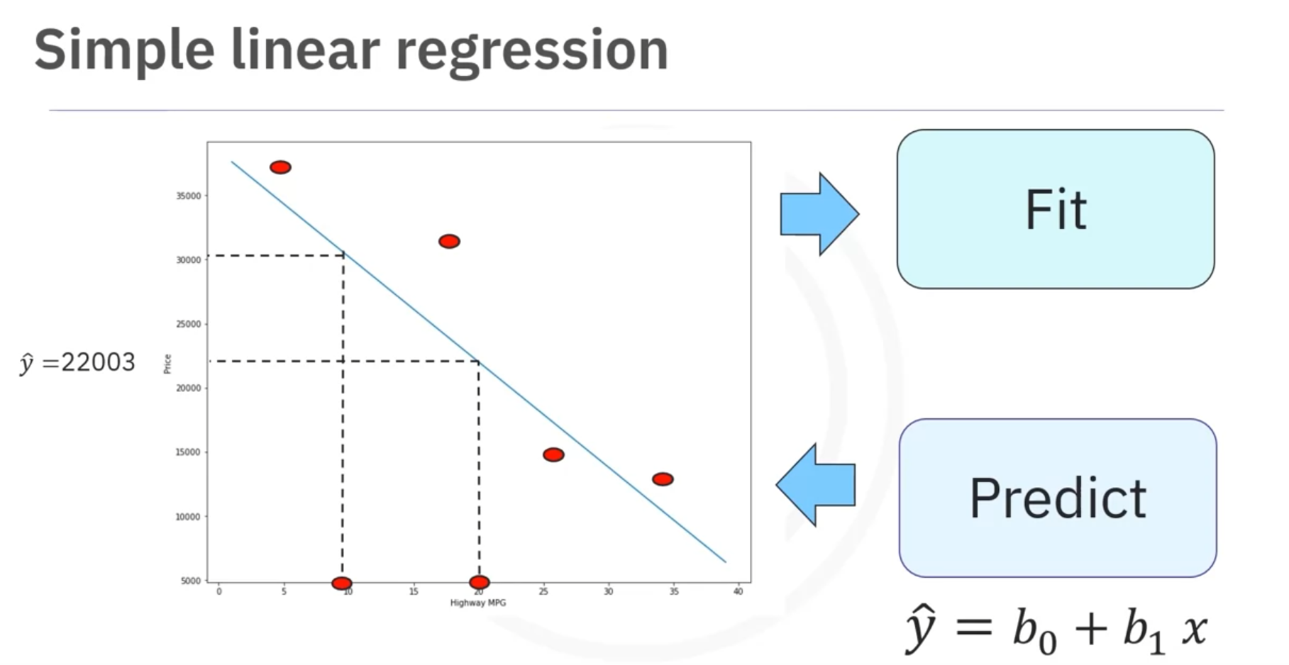

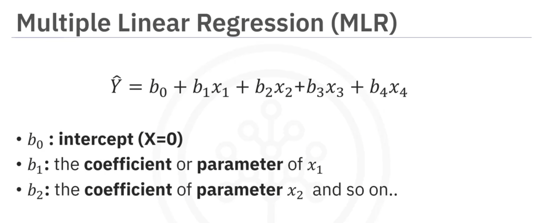
1.2 Multiple Linear Regression (MLR)

Multiple linear regression (MLR) extends SLR to include multiple predictor variables

( $x1,x2, \ldots,xn$ ) to predict a continuous target variable ( $y$ ):

y=b_0+b_1x_1+b_2x_2+...+bn_xn_y

Visualization and Training

With two predictor variables ( $x_1$ and ), data points are mapped on a 2D plane, and () values are mapped vertically.

Python Implementation

from sklearn.linear_model import LinearRegression

# Create a linear regression object
lm = LinearRegression()

# Define predictor variables (z) and target (y)
z = ...
y = ...

# Fit the model
lm.fit(z, y)

# Make predictions
predicted_values = lm.predict(z)

# Model parameters
intercept = lm.intercept_
coefficients = lm.coef_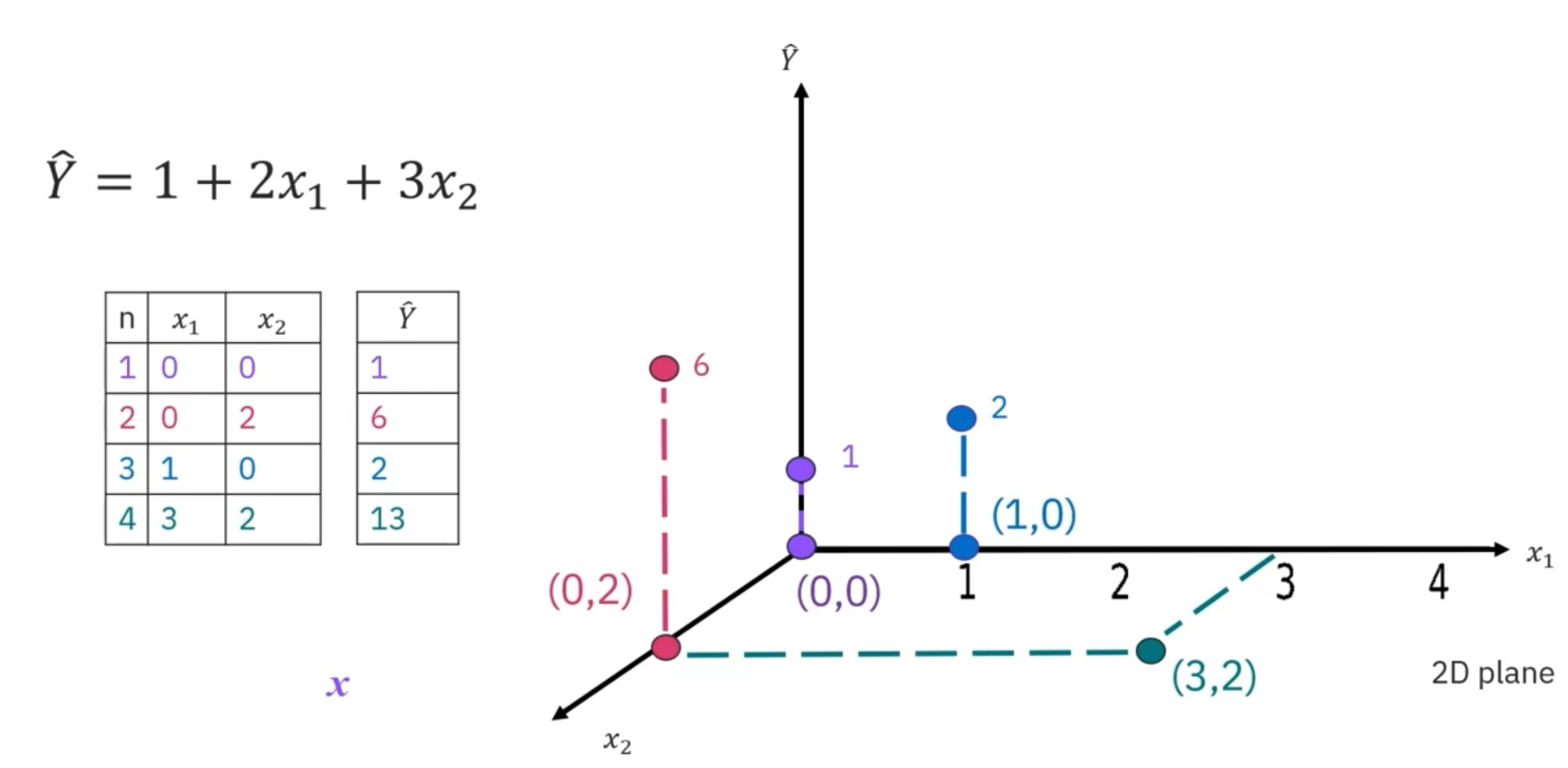

In summary, SLR and MLR provide methods to model relationships between variables, helping predict outcomes based on data observations.

2. Model Evaluation Using Visualization

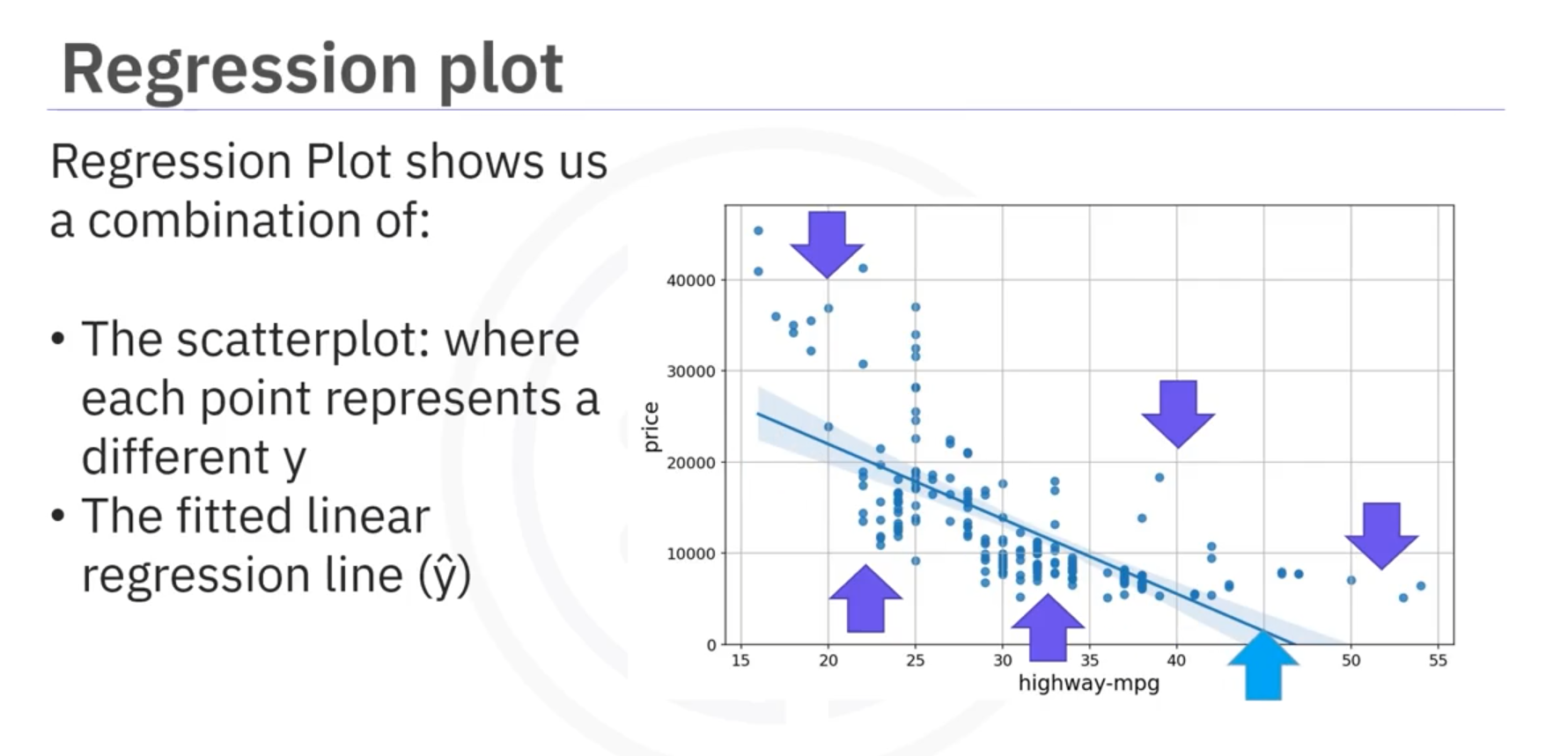
1. Regression Plots

Regression plots estimate the relationship between two variables, showing the strength and direction of the correlation.

Horizontal Axis: Independent variable.

Vertical Axis: Dependent variable.

Points: Represent different target points.

Fitted Line: Represents predicted values.

Creating a Regression Plot

Import Seaborn:
```
import seaborn as sns
```

Use regplot Function:
- Parameters:
  - x: Independent variable column.
  - y: Dependent variable column.
  - data: Name of the DataFrame.
```
sns.regplot(x='feature', y='target', data=df)
```

2. Residual Plots

Residual plots represent the error between actual and predicted values.

Process:
- Subtract predicted value from actual target value.
- Plot the error on the vertical axis, dependent variable on the horizontal axis.

Insights:
- Zero mean distributed evenly around the x-axis indicates a linear model.
- Curvature in residuals suggests a nonlinear model.

Creating a Residual Plot

Import Seaborn:
```
import seaborn as sns
```

Use residplot Function:
- Parameters:
  - Series of dependent variable (feature).
  - Series of target variable.
```
sns.residplot(x='feature', y='target', data=df)
```

3. Distribution Plots

Distribution plots visualize predicted versus actual values.

Use: Helpful for models with multiple independent variables.

Process

Count and plot the predicted points approximately equal to a target value.

Repeat for various target values.

Creating a Distribution Plot

Import Pandas and Seaborn:

import pandas as pd
import seaborn as sns

Use Seaborn's Distribution Plot:
- Parameters:
  - hist: Set to False for a distribution.
  - color: Set to desired color.
  - label: Include label for legend.
```
sns.kdeplot(predicted_values, color='blue', label='Predicted')
sns.kdeplot(actual_values, color='red', label='Actual')
```

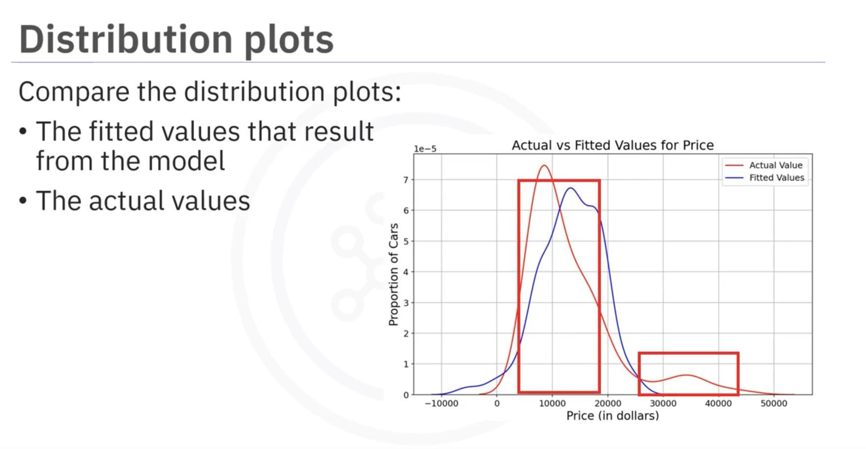
Observation: Prices in range from 40,000 to 50,000 are inaccurate, while 10,000 to 20,000 are closer to target values.

3. Polynomial Regression and Pipelines

Polynomial Regression

What is Polynomial Regression?

Purpose: Used when linear regression isn't suitable.

Approach: Transforms data into polynomial form to capture curvilinear relationships.

Types of Polynomial Models

Quadratic (2nd Order): Includes squared terms.

Cubic (3rd Order): Includes cubed terms.

Higher-Order: Used for complex relationships.

Example Model

3rd Order Polynomial:

−1.557x^3+204.8x^2+8965x+1.37×105

Implementation in Python

Using NumPy:

import numpy as np
coefficients = np.polyfit(x, y, 3)

For Multidimensional:
Use
scikit-learn for more complex models.

Polynomial Features with Scikit-learn

Import the Library:

from sklearn.preprocessing import PolynomialFeatures

Create Polynomial Features:

from sklearn.linear_model import LinearRegression

# Create a PolynomialFeatures object with the desired degree
poly = PolynomialFeatures(degree=3)

# Fit and transform your data
X_poly = poly.fit_transform(X)

# Create LinearRegression model
model = LinearRegression()

# Fit the model with the polynomial features
model.fit(X_poly, y)

In this code:

degree=3 specifies the degree of the polynomial features.

fit_transform(X) generates the polynomial features for your dataset X.

Normalization

Why Normalize?

Purpose: Standardize data for better model performance.

How to Normalize

Using StandardScaler:

from sklearn.preprocessing import StandardScaler
scaler = StandardScaler()
x_scaled = scaler.fit_transform(x)

Pipelines

What are Pipelines?

Purpose: Efficiently automate data preprocessing and model training.

Benefit: Simplifies complex workflows by chaining multiple steps into a single process.

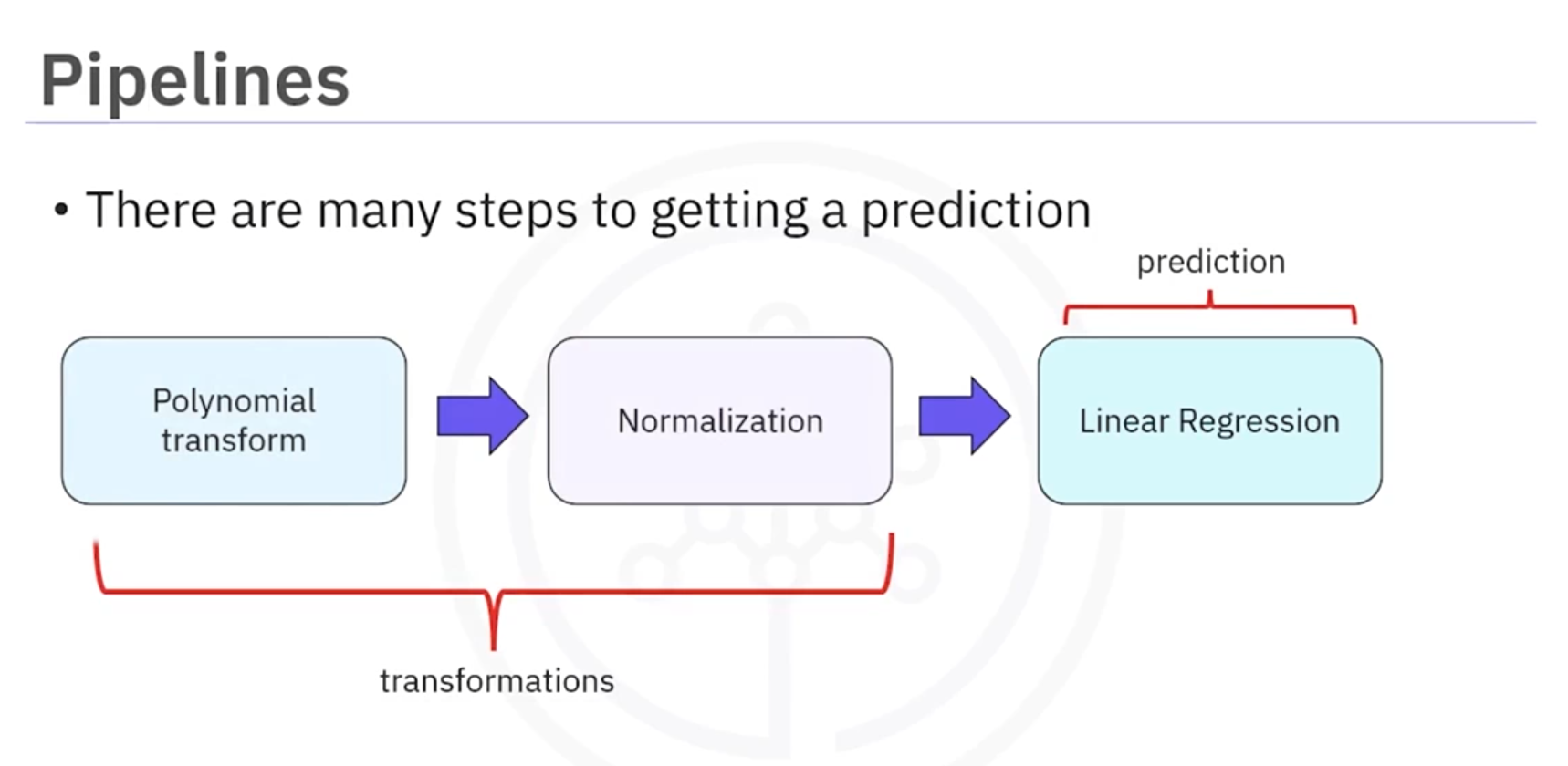
Benefits

Efficiency: Simplifies code by chaining steps.

Maintainability: Makes workflow clearer.

Creating a Pipeline

Import Pipeline:
```
from sklearn.pipeline import Pipeline
```

Define Steps:

pipeline = Pipeline([
    ('scaler', StandardScaler()),
    ('poly', PolynomialFeatures(degree=3)),
    ('model', LinearRegression())
])

Train and Predict:

pipeline.fit(x_train, y_train)
y_pred = pipeline.predict(x_test)

Key Points

Sequential Processing: Automates the flow from preprocessing to prediction.

Versatile: Easily adjust steps and parameters.

Use polynomial regression and pipelines to enhance model accuracy and streamline your machine learning workflow.

Note:

Simple Linear Regression (SLR)

Definition: Models the relationship between two variables by fitting a linear equation.

Equation: $y = b_0 + b_1x$

Use Case: One independent variable predicts a dependent variable.

Multiple Linear Regression (MLR)

Definition: Extends SLR to include multiple independent variables.

Equation: $y=b_0+b_1x_1+b_2x_2+…+b_nx_n$

Use Case: Accounts for multiple factors affecting the outcome.

Polynomial Regression

Definition: A form of regression where the relationship is modeled as an nth degree polynomial.

Equation: $y = b_0 + b_1x + b_2x^2 + \ldots + b_nx^n$

Use Case: Captures non-linear relationships by transforming features.

Key Differences

SLR: Linear relationship with one predictor.

MLR: Linear relationships with multiple predictors.

Polynomial Regression: Non-linear relationships using polynomial terms.

Example Code

from sklearn.linear_model import LinearRegression
from sklearn.preprocessing import PolynomialFeatures
import numpy as np

# Simple Linear Regression
X_slr = np.array([[20], [30], [40]])
y_slr = np.array([15000, 13000, 12000])

model_slr = LinearRegression()
model_slr.fit(X_slr, y_slr)
predicted_slr = model_slr.predict([[30]])
print("SLR Predicted Price:", predicted_slr[0])

# Multiple Linear Regression
X_mlr = np.array([[20, 5], [30, 4], [40, 6]])
y_mlr = np.array([15000, 13000, 12000])

model_mlr = LinearRegression()
model_mlr.fit(X_mlr, y_mlr)
predicted_mlr = model_mlr.predict([[30, 5]])
print("MLR Predicted Price:", predicted_mlr[0])

# Polynomial Regression
X_poly = np.array([[20], [30], [40]])
y_poly = np.array([15000, 13000, 12000])

poly = PolynomialFeatures(degree=2)
X_poly_transformed = poly.fit_transform(X_poly)

model_poly = LinearRegression()
model_poly.fit(X_poly_transformed, y_poly)
predicted_poly = model_poly.predict(poly.transform([[30]]))
print("Polynomial Predicted Price:", predicted_poly[0])

4. Model Evaluation Metrics

Mean Squared Error (MSE)

Definition: Measures the average squared difference between actual and predicted values. It indicates how close predictions are to the actual values.

Formula: $\text{MSE} = \frac{1}{n} \sum (y - \hat{y})^2$

Python: Use mean_squared_error from sklearn.metrics.

Example

Scenario: Predicting house prices based on size.

Actual Prices: [200, 250, 300]

Predicted Prices: [210, 240, 310]

Calculation:

$\text{MSE} = \frac{1}{3} ((200-210)^2 + (250-240)^2 + (300-310)^2) = \frac{1}{3} (100 + 100 + 100) = 100$

Python Code:

from sklearn.metrics import mean_squared_error

actual = [200, 250, 300]
predicted = [210, 240, 310]
mse = mean_squared_error(actual, predicted)
print("MSE:", mse)  # Output: MSE: 100.0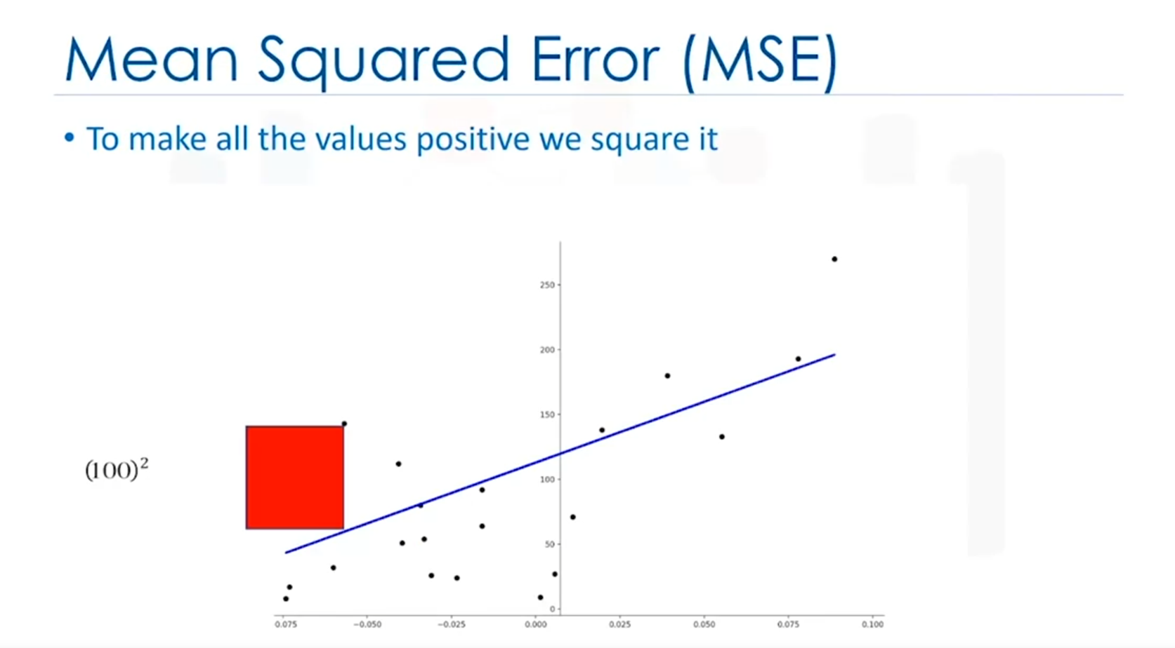

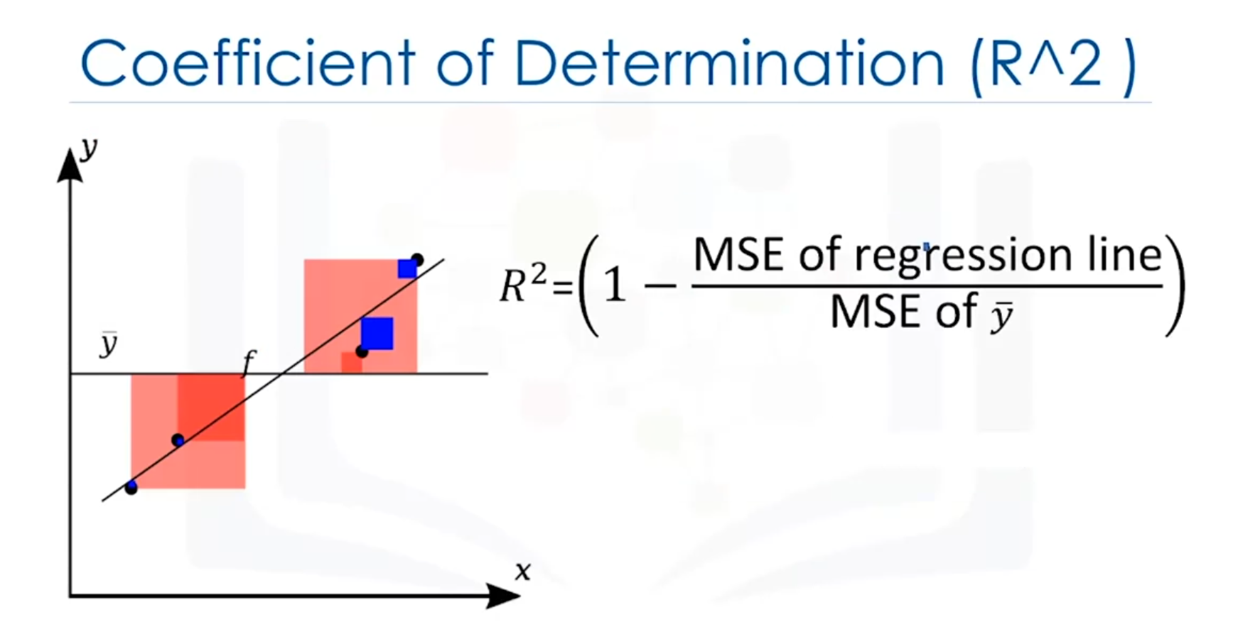
R-squared (Coefficient of Determination)

Definition: Indicates how well the data fits the regression line. Values range from 0 to 1, with values closer to 1 indicating a better fit.

Formula: $R^2 = 1 - \frac{\text{MSE of regression}}{\text{MSE of mean}}$

Python: Use score method in the linear regression object.

Example

Scenario: Predicting test scores based on study hours.

Interpretation:

Good Fit: R² = 0.9 (90% of variance explained)

Poor Fit: R² = 0.2 (20% of variance explained)

Python Code:

from sklearn.linear_model import LinearRegression
import numpy as np

X = np.array([[1], [2], [3]])
y = np.array([2, 3, 5])
model = LinearRegression()
model.fit(X, y)

r_squared = model.score(X, y)
print("R-squared:", r_squared)  # Output: R-squared: 0.9642857142857143

Example Interpretation

Good Fit: Small MSE for regression, larger for mean → $R^2$ near 1.

Poor Fit: Similar MSE for regression and mean → $R^2$ near 0.

Negative $R^2$ : Possible overfitting.

5. Prediction and Decision Making

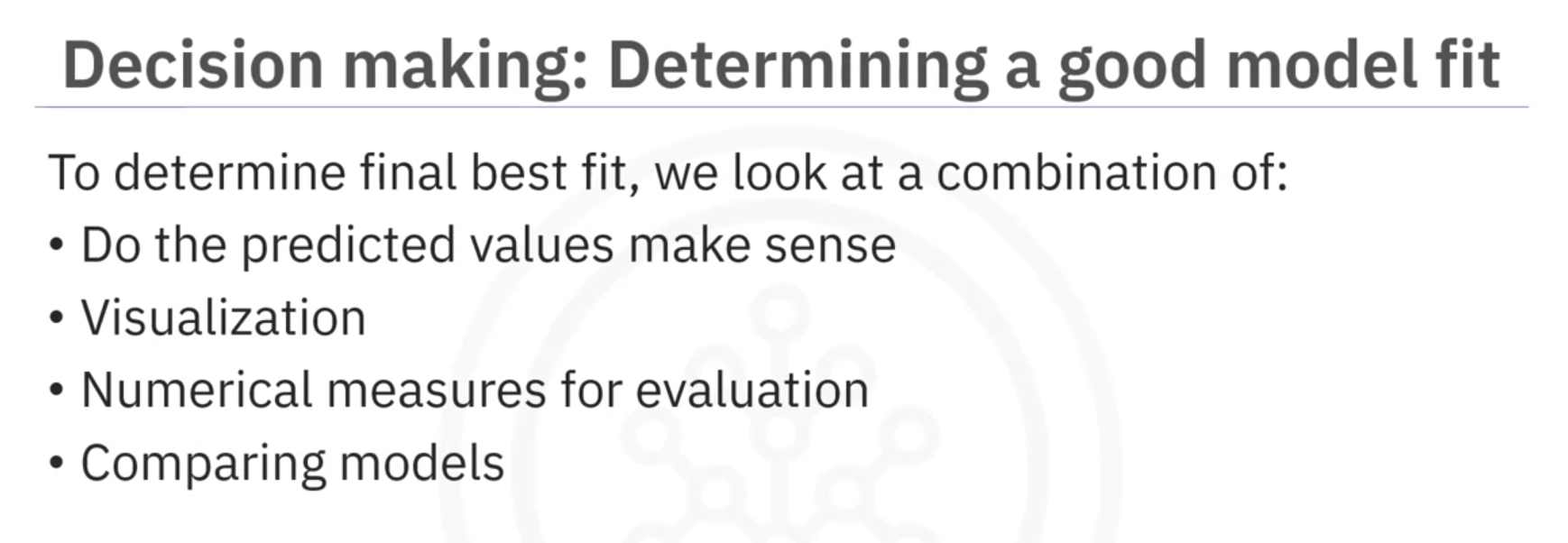
Model Evaluation

To ensure a model's validity, use:

Visualization: Plot data to check trends and anomalies.

Numerical Measures: Metrics like MSE and R-squared.

Comparison: Evaluate different models.

Example: Predicting Car Price

Scenario: Predict price for a car with 30 highway mpg.

Result: Price = $13,771.30 (reasonable value).

Coefficient Interpretation

An increase of 1 mpg decreases price by $821.

Potential Issues

Unrealistic predictions may indicate:

Incorrect assumptions

Lack of data in certain ranges

Generating Predictions

Use NumPy's arange to create sequences for prediction.

import numpy as np
from sklearn.linear_model import LinearRegression

# Sample data
X = np.array([[20], [30], [40]])
y = np.array([15000, 13000, 12000])

# Model training
model = LinearRegression()
model.fit(X, y)

# Generating a sequence for prediction
mpg_values = np.arange(1, 101, 1)  # From 1 to 100 with step 1
predicted_prices = model.predict(mpg_values.reshape(-1, 1))

# Example prediction for 30 mpg
predicted_price = model.predict([[30]])
print("Predicted Price:", predicted_price[0])

Explanation

np.arange(1, 101, 1): Creates an array from 1 to 100 with a step of 1.

reshape(-1, 1): Reshapes the array for prediction.

Visualization Techniques

Regression Plot: Shows data trend and potential non-linear behavior.

Residual Plot: Curvature indicates non-linear relationships.

Distribution Plot: Highlights prediction accuracy in certain ranges.

Evaluating Models

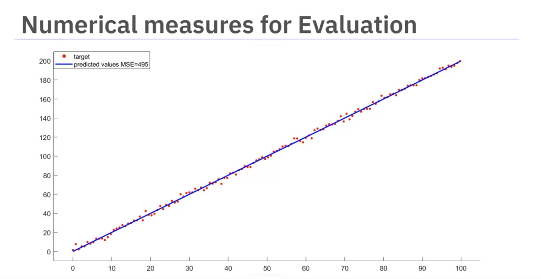
Mean Squared Error (MSE)

Interpretation: Average squared difference between actual and predicted values.

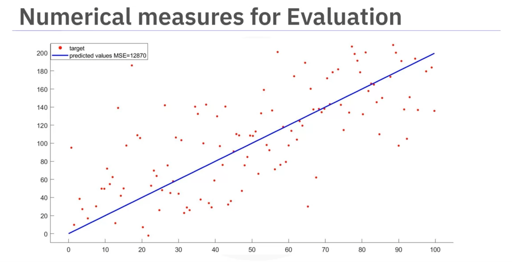
Example MSEs:

495 (good fit)

12,870 (poor fit)

Code Example:

from sklearn.metrics import mean_squared_error

# Actual and predicted values
actual = [15000, 13000, 12000]
predicted = model.predict(X)

# Calculate MSE
mse = mean_squared_error(actual, predicted)
print("MSE:", mse)

R-squared (R²)

Definition: Indicates how well data fits the regression line.

Example R² Values:

0.9986 (excellent fit)

0.61 (weak linear relation)

# Calculate R-squared
r_squared = model.score(X, y)
print("R-squared:", r_squared)

Model Comparison

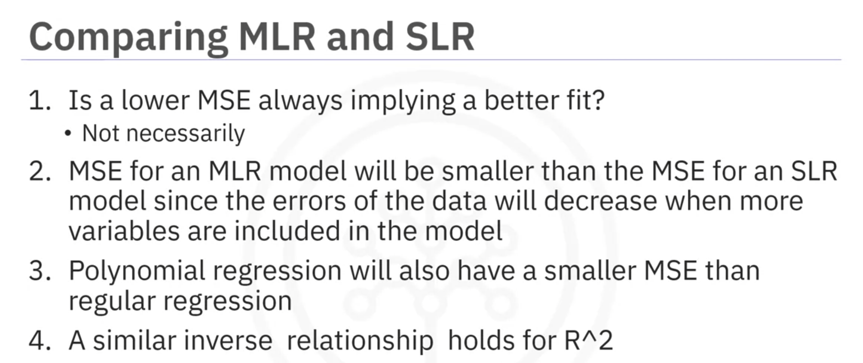
MLR vs. SLR: More variables can lower MSE, but not always a better fit.

Polynomial Regression: Generally has lower MSE compared to linear regression.

Conclusion

Evaluate models using both visualization and numerical metrics.

Consider context and domain for interpreting R² and MSE values.

Notes

Regression Plot

When it comes to simple linear regression, an excellent way to visualize the fit of our model is by using regression plots.

This plot will show a combination of scattered data points (a scatterplot), as well as the fitted linear regression line going through the data. This will give us a reasonable estimate of the relationship between the two variables, the strength of the correlation, as well as the direction (positive or negative correlation).

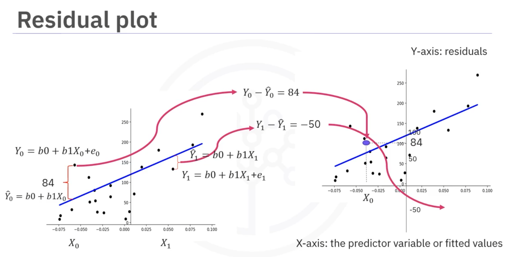
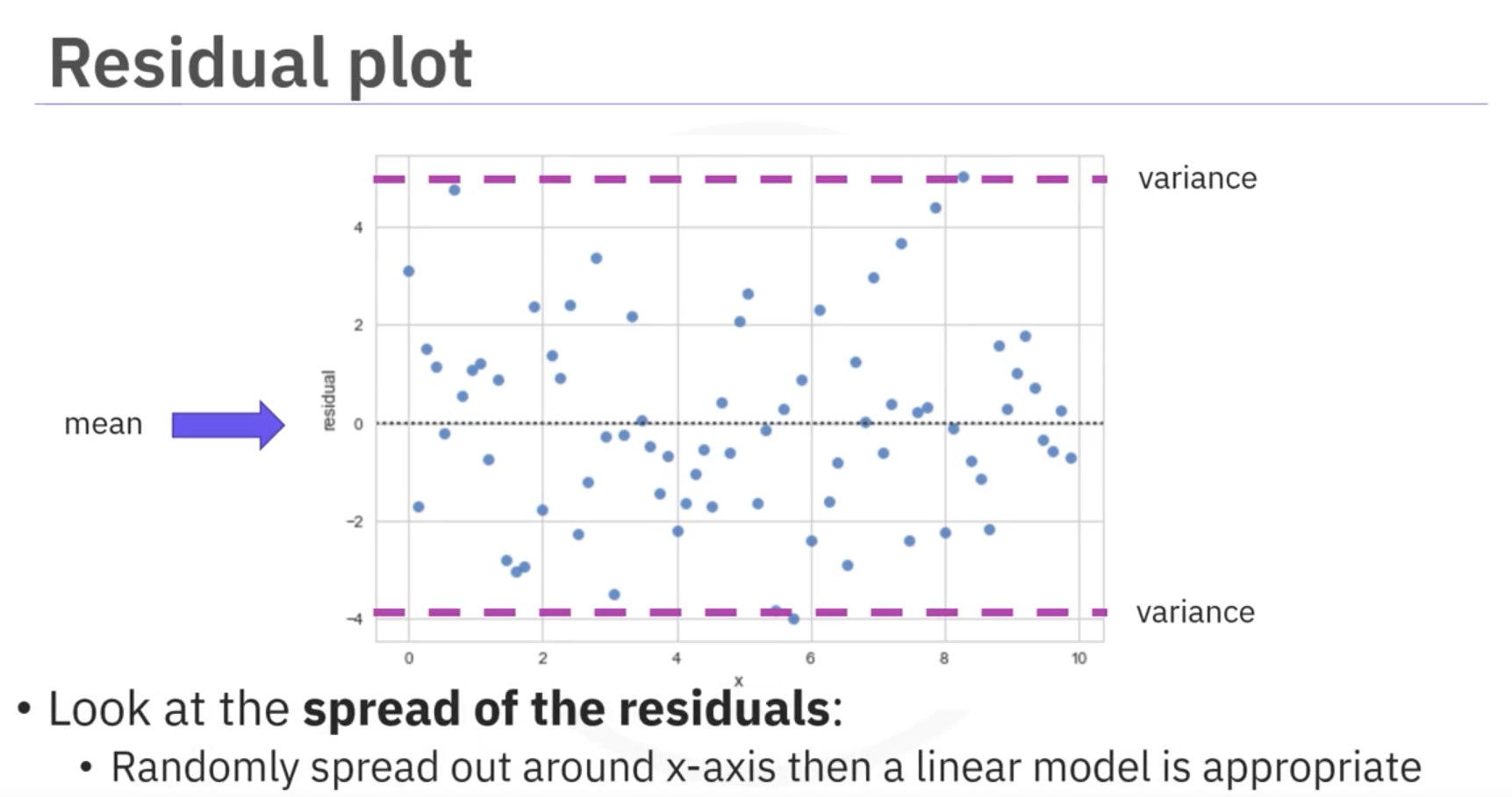
Residual Plot

A good way to visualize the variance of the data is to use a residual plot.

What is a residual?

The difference between the observed value (y) and the predicted value (ŷ) is called the residual (e). When we look at a regression plot, the residual is the distance from the data point to the fitted regression line.

So what is a residual plot?

A residual plot is a graph that shows the residuals on the vertical y-axis and the independent variable on the horizontal x-axis.

What do we pay attention to when looking at a residual plot?

We look at the spread of the residuals:

If the points in a residual plot are randomly spread out around the x-axis, then a linear model is appropriate for the data.

Why is that? Randomly spread out residuals mean that the variance is constant, and thus the linear model is a good fit for this data.

Simple Linear Regression

One example of a Data Model that we will be using is Simple Linear Regression.

Simple Linear Regression is a method to help us understand the relationship between two variables:

The predictor/independent variable (X)

The response/dependent variable (that we want to predict) (Y)

The result of Linear Regression is a linear function that predicts the response (dependent) variable as a function of the predictor (independent) variable.

Multiple Linear Regression

What if we want to predict car price using more than one variable?

If we want to use more variables in our model to predict car price, we can use Multiple Linear Regression. Multiple Linear Regression is very similar to Simple Linear Regression, but this method is used to explain the relationship between one continuous response (dependent) variable and two or more predictor (independent) variables. Most of the real-world regression models involve multiple predictors. We will illustrate the structure by using four predictor variables, but these results can generalize to any number.

Polynomial Regression

Polynomial regression is a particular case of the general linear regression model or multiple linear regression models.

We get non-linear relationships by squaring or setting higher-order terms of the predictor variables.

Measures for In-Sample Evaluation

When evaluating our models, not only do we want to visualize the results, but we also need a quantitative measure to determine how accurate the model is.

Two very important measures that are often used in statistics to assess the accuracy of a model are:

R² / R-squared (The Coefficient of Determination)

Mean Squared Error (MSE)

R-squared

R-squared, also known as the coefficient of determination, measures how closely the data aligns with the fitted regression line.

The R-squared value represents the percentage of variation in the response variable (y) that is explained by the linear model.

Mean Squared Error (MSE)

The Mean Squared Error (MSE) measures the average of the squares of the errors. In other words, it calculates the difference between the actual values (y) and the estimated values (ŷ).

Cheat Sheet: Model Development

Linear Regression

Process: Create a Linear Regression model object

Description: Create an instance of the LinearRegression model.

Code Example:

from sklearn.linear_model import LinearRegression

lr = LinearRegression()

Train Linear Regression Model

Process: Train the Linear Regression model

Description: Fit the model on the input and output data. If there’s only one input attribute, it’s simple linear regression. If there are multiple attributes, it’s multiple linear regression.

Code Example:

X = df[['attribute_1', 'attribute_2', ...]]
Y = df['target_attribute']

lr.fit(X, Y)

Generate Output Predictions

Process: Predict the output for given input attributes

Description: Use the trained model to predict the output values based on the input attributes.

Code Example:
```
Y_hat = lr.predict(X)
```

Identify the Coefficient and Intercept

Process: Retrieve the model’s coefficient and intercept

Description: Access the slope coefficient and intercept values of the linear regression model.

Code Example:

coeff = lr.coef_
intercept = lr.intercept_

Residual Plot

Process: Create a Residual Plot

Description: Plot the residuals (the differences between observed and predicted values) to assess the goodness of fit.

Code Example:

import seaborn as sns

sns.residplot(x=df['attribute_1'], y=df['attribute_2'])

Distribution Plot

Process: Create a Distribution Plot

Description: Plot the distribution of a given attribute’s data.

Code Example:

import seaborn as sns

sns.distplot(df['attribute_name'], hist=False)

Polynomial Regression

Process: Perform Polynomial Regression

Description: Fit a polynomial model to the data using NumPy.

Code Example:

import numpy as np

f = np.polyfit(x, y, n)
p = np.poly1d(f)
Y_hat = p(x)

Multi-variate Polynomial Regression

Process: Create Polynomial Features

Description: Generate polynomial combinations of features up to a specified degree.

Code Example:

from sklearn.preprocessing import PolynomialFeatures

Z = df[['attribute_1', 'attribute_2', ...]]
pr = PolynomialFeatures(degree=n)
Z_pr = pr.fit_transform(Z)

Pipeline

Process: Create a Data Pipeline

Description: Simplify the steps of processing data by creating a pipeline with a sequence of steps.

Code Example:

from sklearn.pipeline import Pipeline
from sklearn.preprocessing import StandardScaler
from sklearn.preprocessing import PolynomialFeatures
from sklearn.linear_model import LinearRegression

Input = [
    ('scale', StandardScaler()),
    ('polynomial', PolynomialFeatures(include_bias=False)),
    ('model', LinearRegression())
]
pipe = Pipeline(Input)
Z = Z.astype(float)
pipe.fit(Z, y)
ypipe = pipe.predict(Z)

R² Value

Process: Calculate R² Value

Description: Measure how well the model’s predictions fit the data. This is the proportion of variance explained by the model.

Code Example:

For Linear Regression:

from sklearn.metrics import r2_score

R2_score = lr.score(X, Y)

For Polynomial Regression:

from sklearn.metrics import r2_score
import numpy as np

f = np.polyfit(x, y, n)
p = np.poly1d(f)
R2_score = r2_score(y, p(x))

Mean Squared Error (MSE) Value

Process: Calculate Mean Squared Error (MSE)

Description: Measure the average of the squares of the errors, which are the differences between actual values and the estimated values.

Code Example:

from sklearn.metrics import mean_squared_error

MSE = mean_squared_error(Y, Y_hat)