Model Evaluation

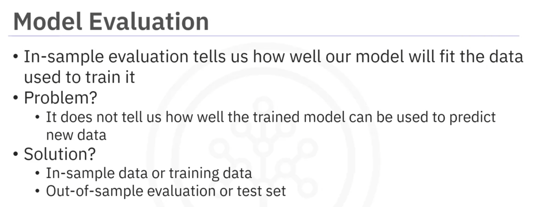
In-Sample vs. Out-of-Sample Evaluation

• In-Sample Evaluation: Measures how well the model fits the training data. It does not estimate how well the model will perform on new, unseen data.

• Out-of-Sample Evaluation: Assesses how the model performs on new data. This is achieved by splitting the data into training and testing sets.

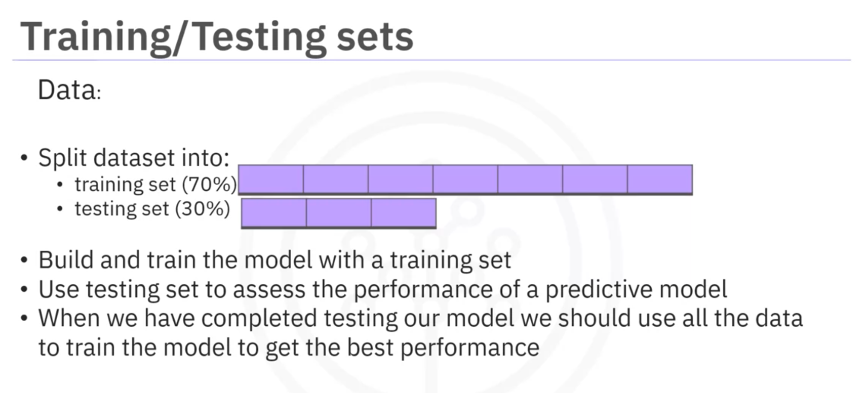
Data Splitting

1. Training Data: Used to build and train the model. Typically, a larger portion of the dataset.

2. Testing Data: Used to evaluate the model's performance. Usually, a smaller portion of the dataset, such as 30%.

Example Code:

from sklearn.model_selection import train_test_split

# Split the data into training and testing sets
X_train, X_test, y_train, y_test = train_test_split(X, y, test_size=0.3, random_state=42)

# X_train: Training data for the predictors
# X_test: Testing data for the predictors
# y_train: Training data for the target variable
# y_test: Testing data for the target variable
# test_size=0.3: 30% of the data will be used for testing, and 70% will be used for training
# random_state=42:Ensures reproducibility of the split. Using the same random state will produce the same split every time

Generalization Error

• Generalization Error: Measures how well the model predicts new data. The error obtained using testing data approximates this error.

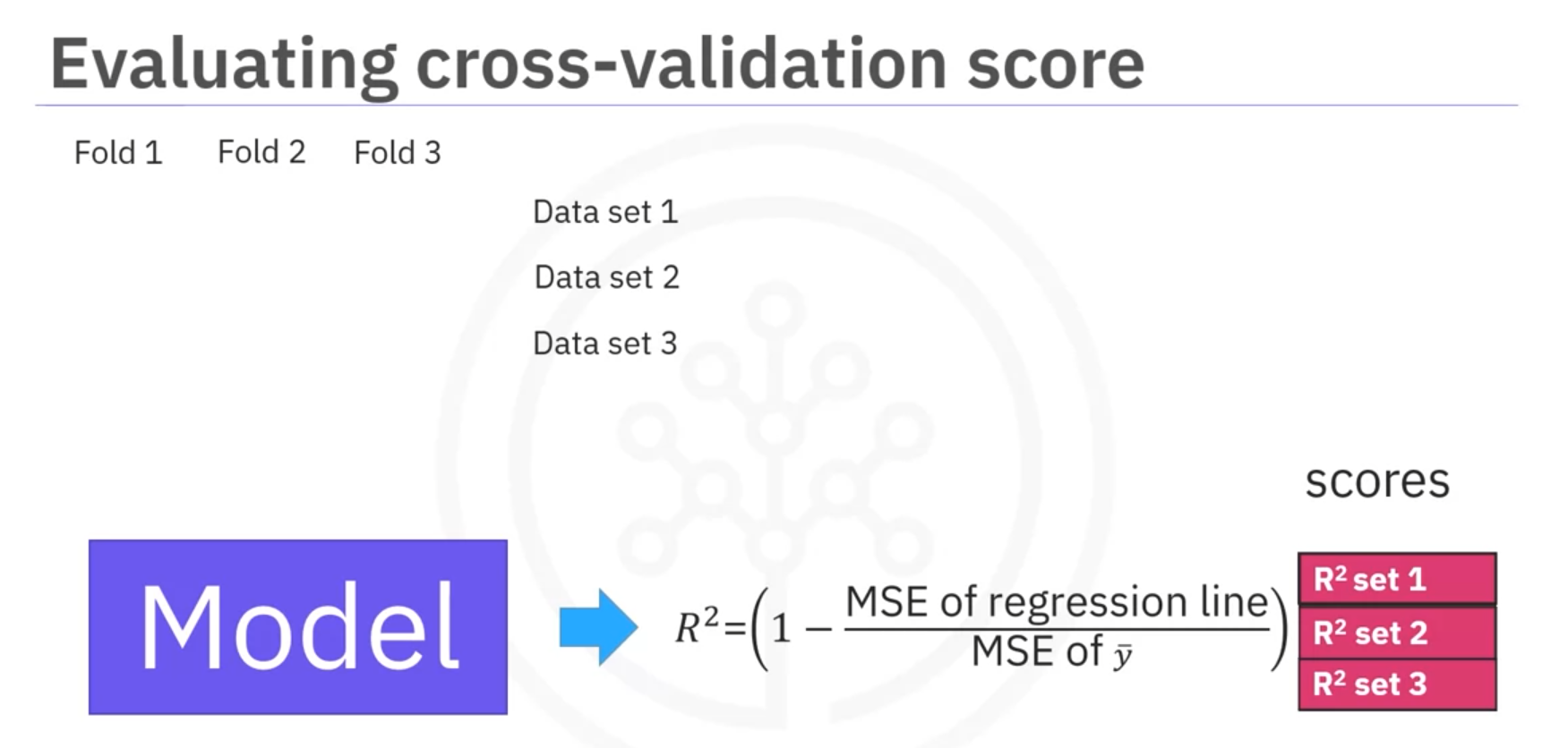
Cross-Validation

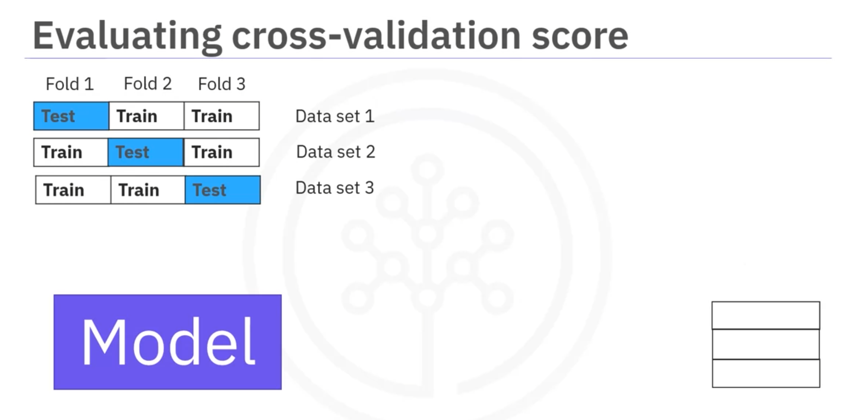
Cross-Validation: A technique to assess the model's performance and estimate generalization error by splitting the data into multiple folds.

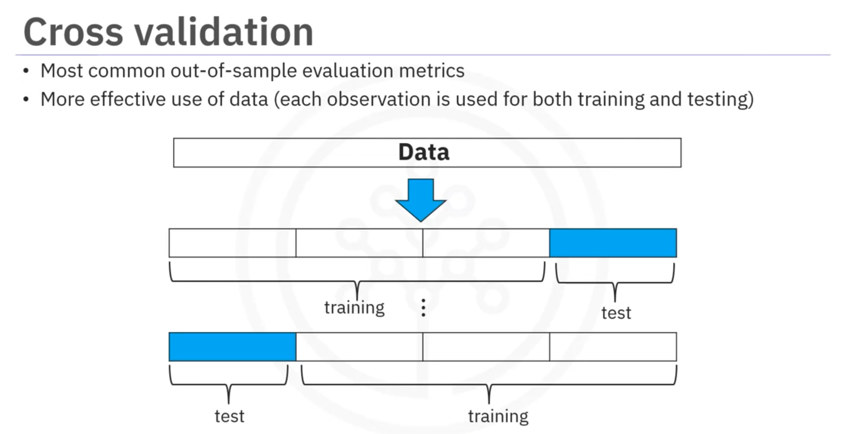
1. Splitting Data: The dataset is divided into k equal parts (folds). Each fold is used once as a testing set while the remaining k − 1 folds are used as the training set.

2. Using cross_val_score:

   from sklearn.model_selection import cross_val_score
   from sklearn.linear_model import LinearRegression
   
   model = LinearRegression()
   scores = cross_val_score(model, X, y, cv=3)  # 3-fold cross-validation
   mean_score = np.mean(scores)

Cross-Val Predict

cross_val_predict is used when you want to obtain the predicted values for each test fold during the cross-validation process. It returns the prediction for each data point when it was in the test set. This is useful for:

1. Visualizing Predictions: You can plot the predicted values against the actual values to see how well the model performs across the entire dataset.

2. Diagnostics: It helps in analyzing the residuals (differences between actual and predicted values) to diagnose model performance.

Example in Python

Here's an example using cross_val_predict:

from sklearn.model_selection import cross_val_predict
from sklearn.linear_model import LinearRegression
import numpy as np
import matplotlib.pyplot as plt

# Example dataset
X = np.random.rand(100, 5)
y = np.random.rand(100)

# Initialize the model
model = LinearRegression()

# Get cross-validated predictions
y_pred = cross_val_predict(model, X, y, cv=5)

# Plot actual vs. predicted values
plt.scatter(y, y_pred)
plt.xlabel('Actual Values')
plt.ylabel('Predicted Values')
plt.title('Cross-Validated Predictions')
plt.show()

In this example:

• cross_val_predict returns the predicted values for each test fold during the 5-fold cross-validation.

• A scatter plot is created to visualize the actual vs. predicted values.

Summary

• Training Set: Used to build the model.

• Testing Set: Used to evaluate model performance.

• Cross-Validation: Provides a robust estimate of model performance by averaging results across multiple folds.

Model Selection and Polynomial Regression

When selecting the best polynomial order, our goal is to provide the best estimate of the

function $y(x)$.

Noise in Data

Noise in data refers to random variations or errors that obscure the true underlying patterns or relationships. It can come from various sources and affects the accuracy of models.

Underfitting

Underfitting occurs when the model is too simple to fit the data:

• Example: Fitting a linear function to data generated from a higher-order polynomial plus noise results in many errors.

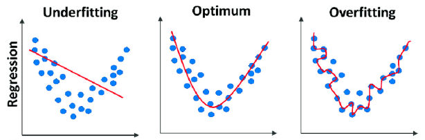
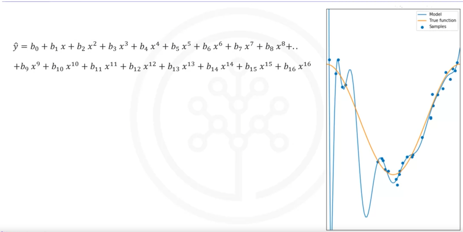
Overfitting

Overfitting occurs when the model is too flexible and fits the noise rather than the function:

• Example: Using a 16th order polynomial, the model does well on training data but performs poorly at estimating the function, especially where there is little training data.

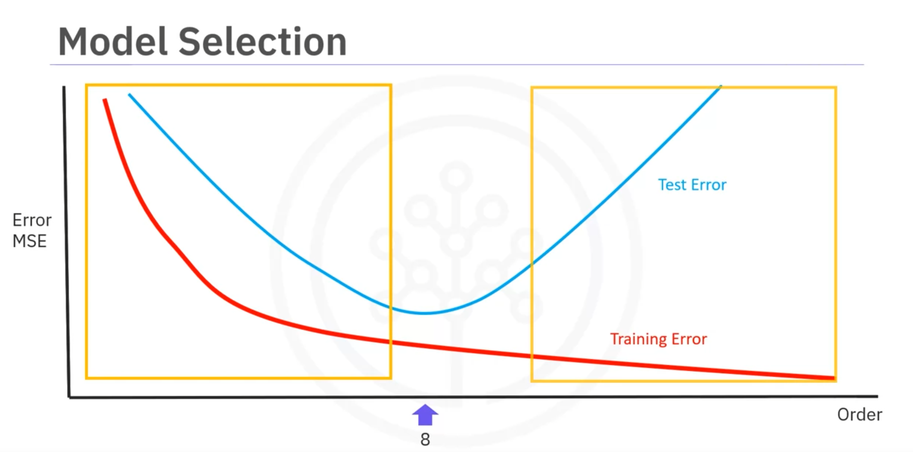
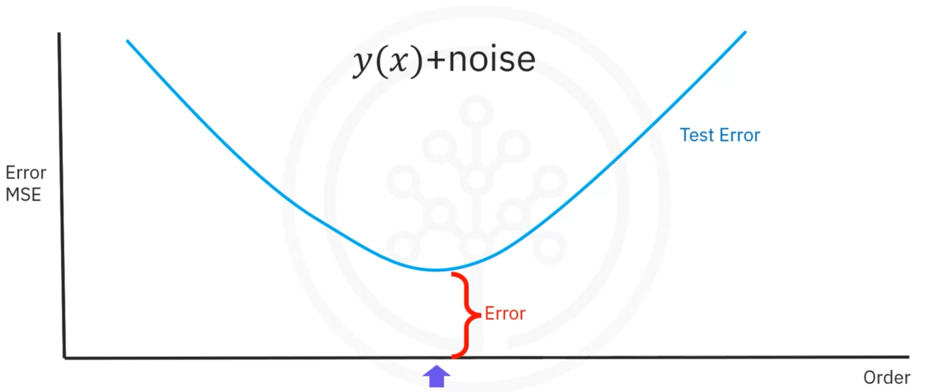
Optimal Polynomial Order

• To determine the best order, we use the mean square error (MSE) for training and testing sets.

• The best order minimizes the test error.

• Errors on the left indicate underfitting, while errors on the right indicate overfitting.

Irreducible Error

• Noise in the data contributes to the error, which is unpredictable and cannot be reduced.

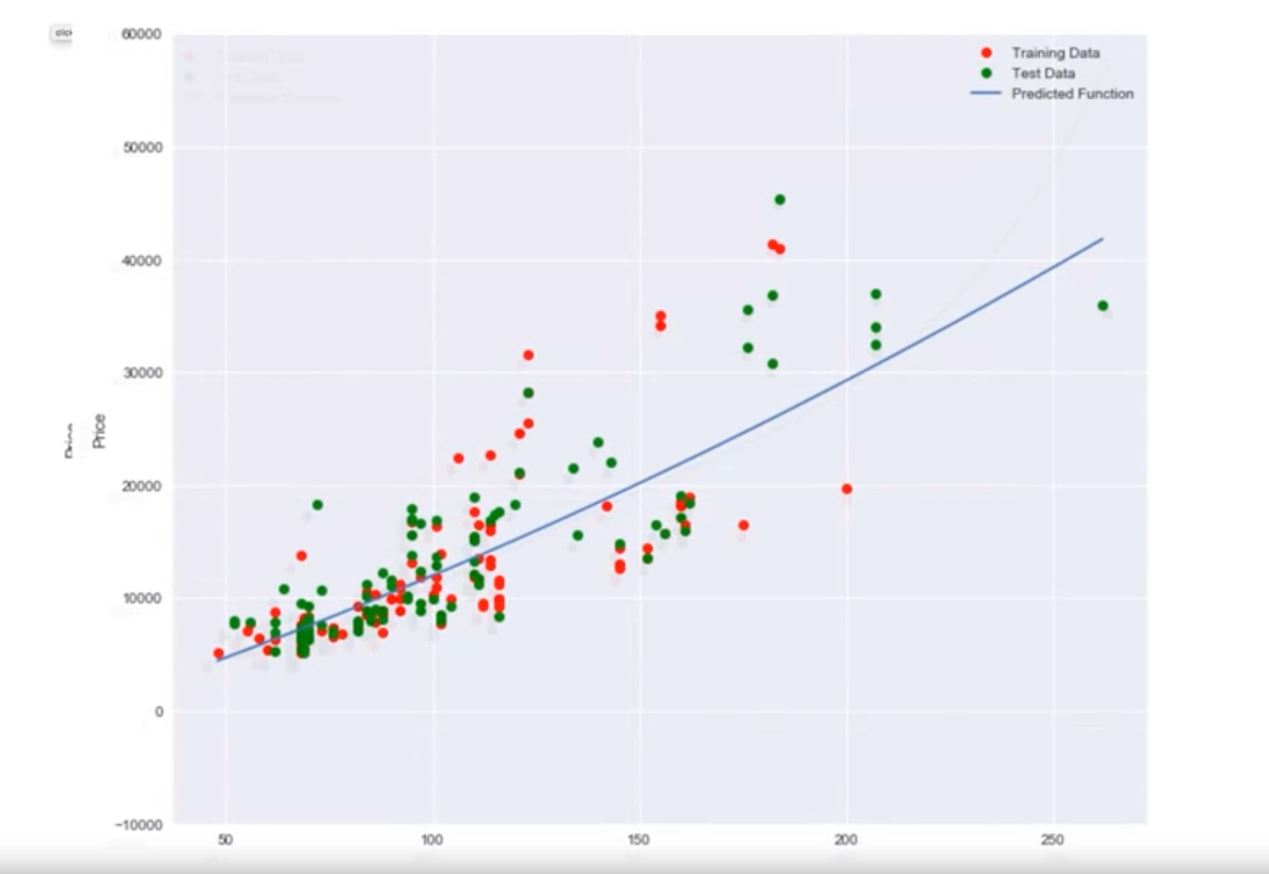
Example with Real Data

• When using horsepower data:
  • A linear function fits the data better than just using the mean.

  

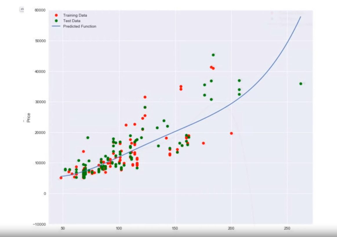
  • A second and third order polynomial improve the fit.

  

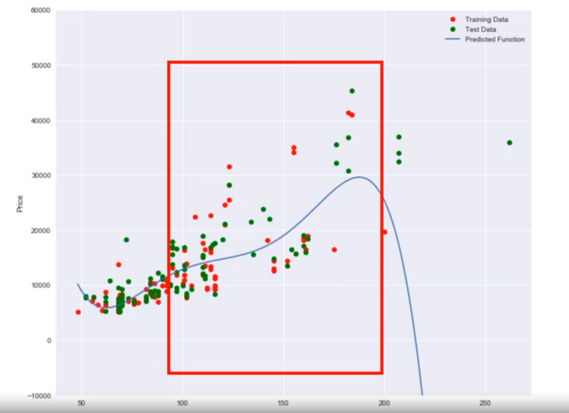
  • A fourth order polynomial shows erroneous behavior.

  

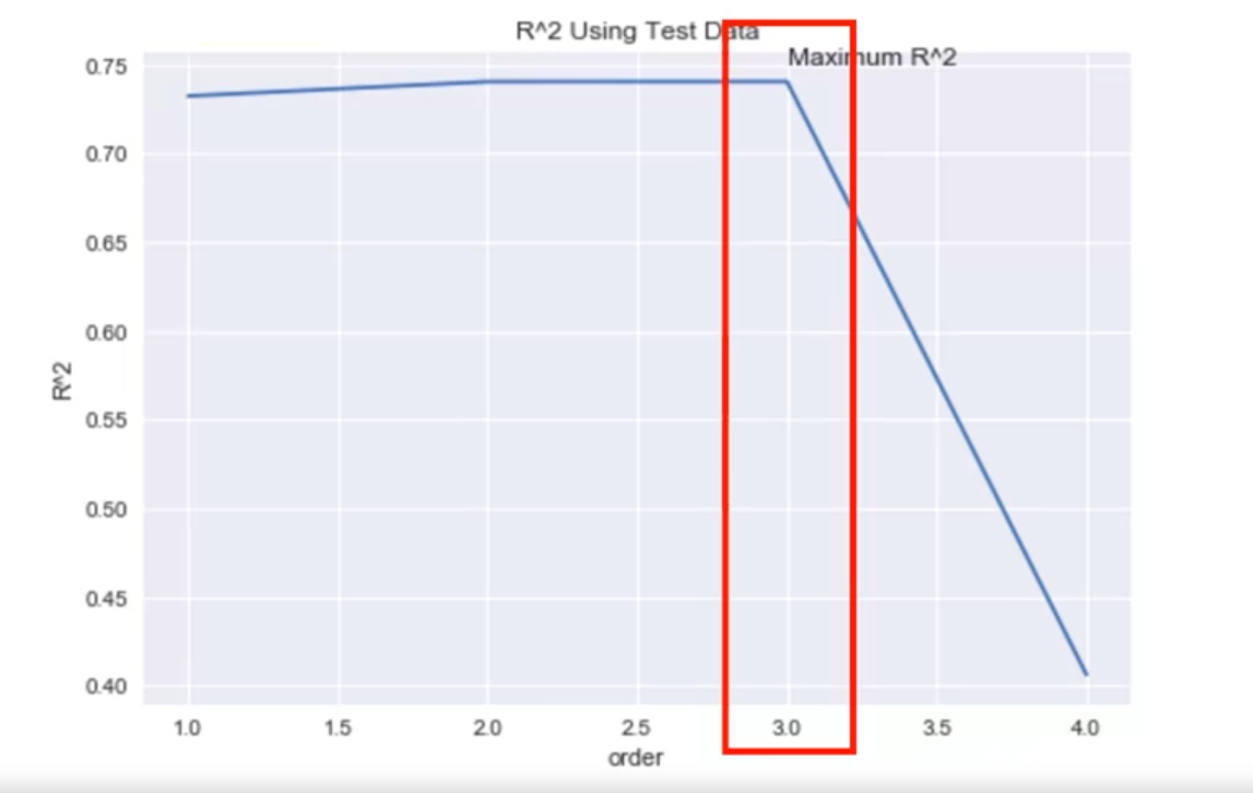
R-squared Analysis

• Plot the R^2 value against the order of polynomial models.

• The optimal order has an R^2 close to one.

• A drastic decrease in R^2 beyond the optimal order indicates overfitting.

Calculating R-squared Values

1. Create an empty list to store R^2 values.

2. Create a list of different polynomial orders.

3. Iterate through the list using a loop:
   • Create a polynomial feature object with the order as a parameter.
   • Transform the training and test data into polynomial features using the fit_transform method.
   • Fit the regression model using the transformed data.
   • Calculate the R^2 value using the test data and store it in the list.

Here's an example of how you can implement this in Python:

import numpy as np
import matplotlib.pyplot as plt
from sklearn.preprocessing import PolynomialFeatures
from sklearn.linear_model import LinearRegression
from sklearn.metrics import r2_score

# Sample data
x = np.array([1, 2, 3, 4, 5])
y = np.array([1, 4, 9, 16, 25])

# Store R^2 values
r2_values = []

# List of polynomial orders
orders = [1, 2, 3, 4]

# Iterate through polynomial orders
for order in orders:
    # Create polynomial features
    poly = PolynomialFeatures(degree=order)
    x_poly = poly.fit_transform(x.reshape(-1, 1))

    # Fit the model
    model = LinearRegression()
    model.fit(x_poly, y)

    # Predict and calculate R^2
    y_pred = model.predict(x_poly)
    r2 = r2_score(y, y_pred)
    r2_values.append(r2)

# Plot R^2 values
plt.plot(orders, r2_values, marker='o')
plt.xlabel('Order of Polynomial')
plt.ylabel('R^2 Value')
plt.title('R^2 Value vs. Polynomial Order')
plt.show()

Output:

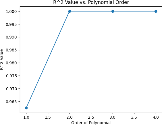
This process helps in identifying the best polynomial order that minimizes the generalization error and avoids underfitting or overfitting.

Introduction to Ridge Regression

For models with multiple independent features and ones with polynomial feature extrapolation, it is common to have colinear combinations of features. Left unchecked, this multicollinearity of features can lead the model to overfit the training data. To control this, the feature sets are typically regularized using hyperparameters.

Ridge regression is the process of regularizing the feature set using the hyperparameter alpha Ridge regression can be utilized to regularize and reduce standard errors and avoid over-fitting while using a regression model.

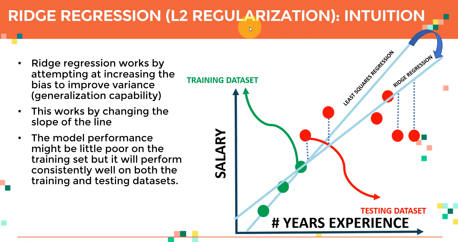
Ridge Regression

Overview: Ridge regression is a technique used to prevent overfitting in polynomial regression by controlling the magnitude of polynomial coefficients.

Key Concepts

1. Overfitting:
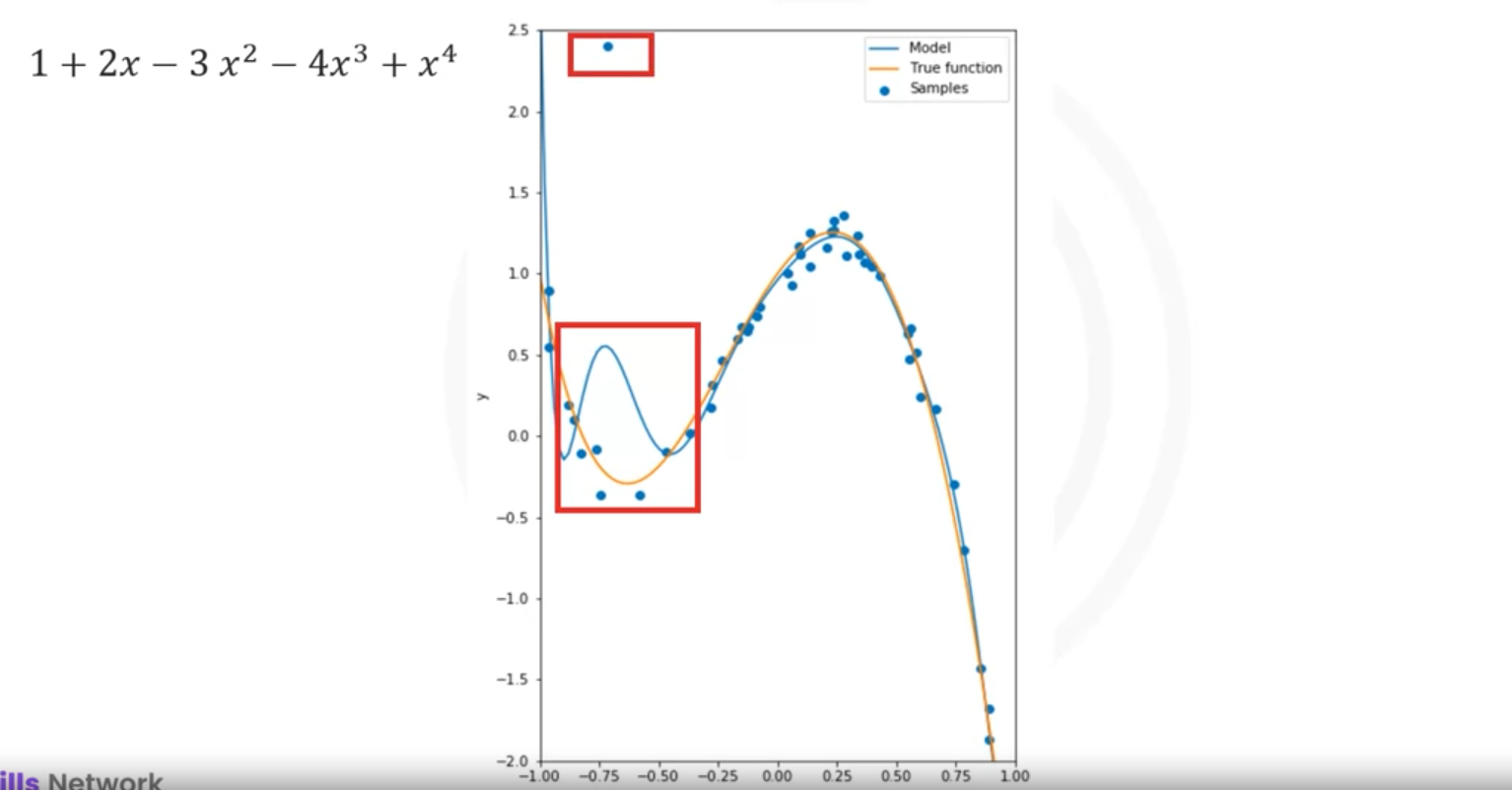
   • Problem: Higher-order polynomials can fit training data very well, but might overfit, especially in the presence of outliers or noisy data.
   • Example: A 10th-order polynomial fitting data with an outlier may produce large coefficients, which can misrepresent the true function.

   

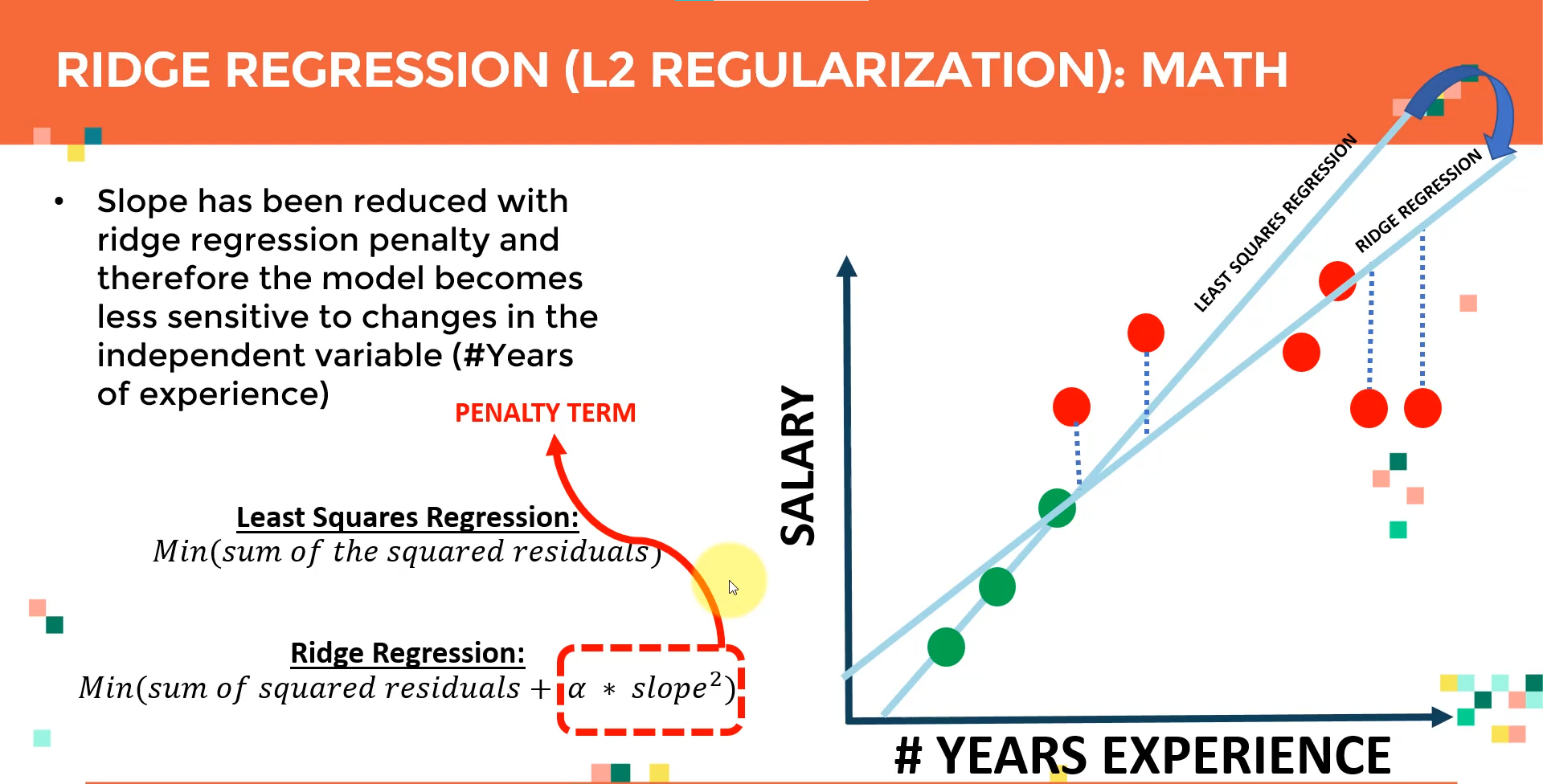
2. Ridge Regression:
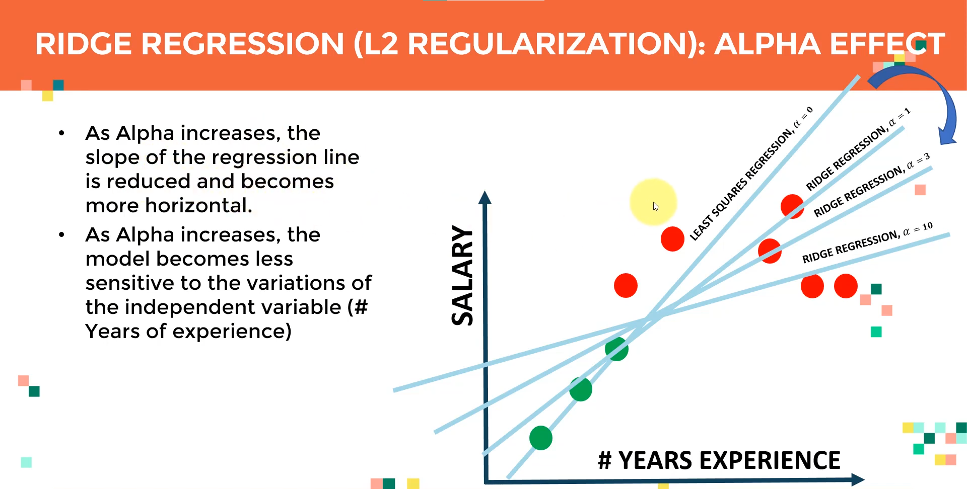
   • Purpose: Ridge regression addresses overfitting by introducing a parameter, Alpha ($\alpha$), which penalizes large coefficients.
   • Effect: As Alpha increases, the magnitude of the coefficients decreases, which can prevent overfitting.
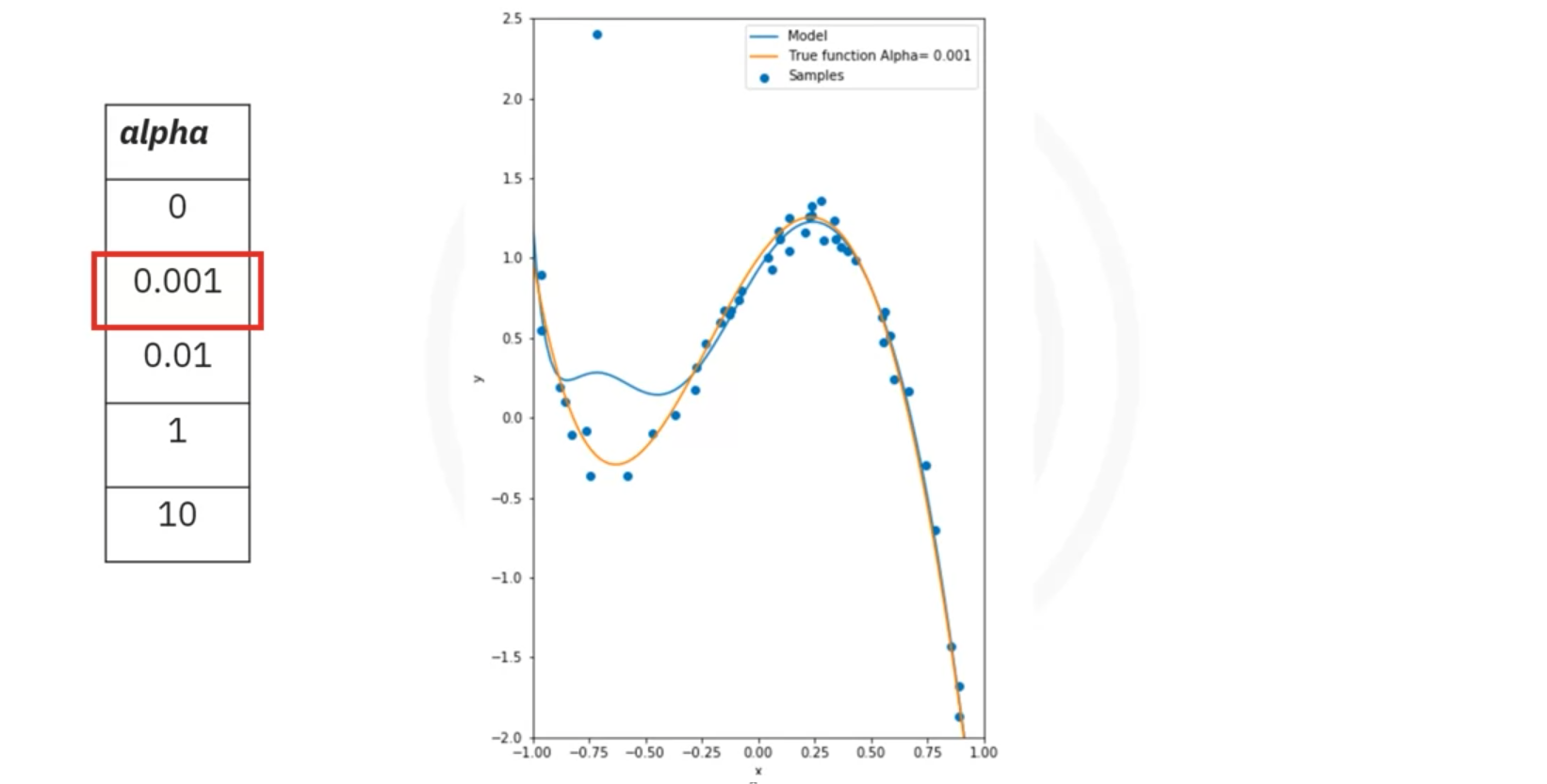
   • Alpha Selection:
     • Too Small Alpha: Might still overfit the data.

     

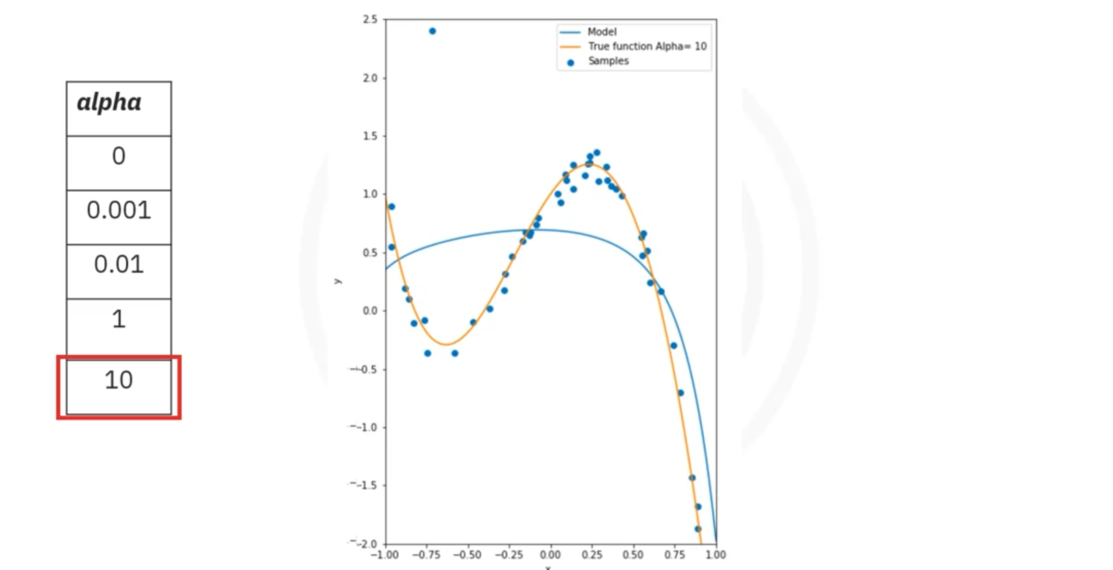
     • Too Large Alpha: Can lead to underfitting as the model becomes too simple.

     

3. Model Training:
   • Procedure: Use cross-validation to select the optimal Alpha. Split the data into training and validation sets.
   • Steps:
     1. Train Model: Fit the model using different values of Alpha.
     2. Predict & Evaluate: Use validation data to make predictions and calculate the R^2 or other metrics.
     3. Select Alpha: Choose the Alpha that maximizes the R^2 on validation data.

4. Implementation in Python:
   • Import:

     from sklearn.linear_model import Ridge

   • Create & Fit Model:

     ridge = Ridge(alpha=1.0)  # Set the desired alpha value
     ridge.fit(X_train, y_train)

   • Predict:

     y_pred = ridge.predict(X_test)

5. Cross-Validation:
   • Purpose: Used to determine the best Alpha by comparing performance metrics (e.g., R^2) across different Alpha values.
   • Process: Train with various Alpha values, evaluate with validation data, and select the best-performing Alpha.

   

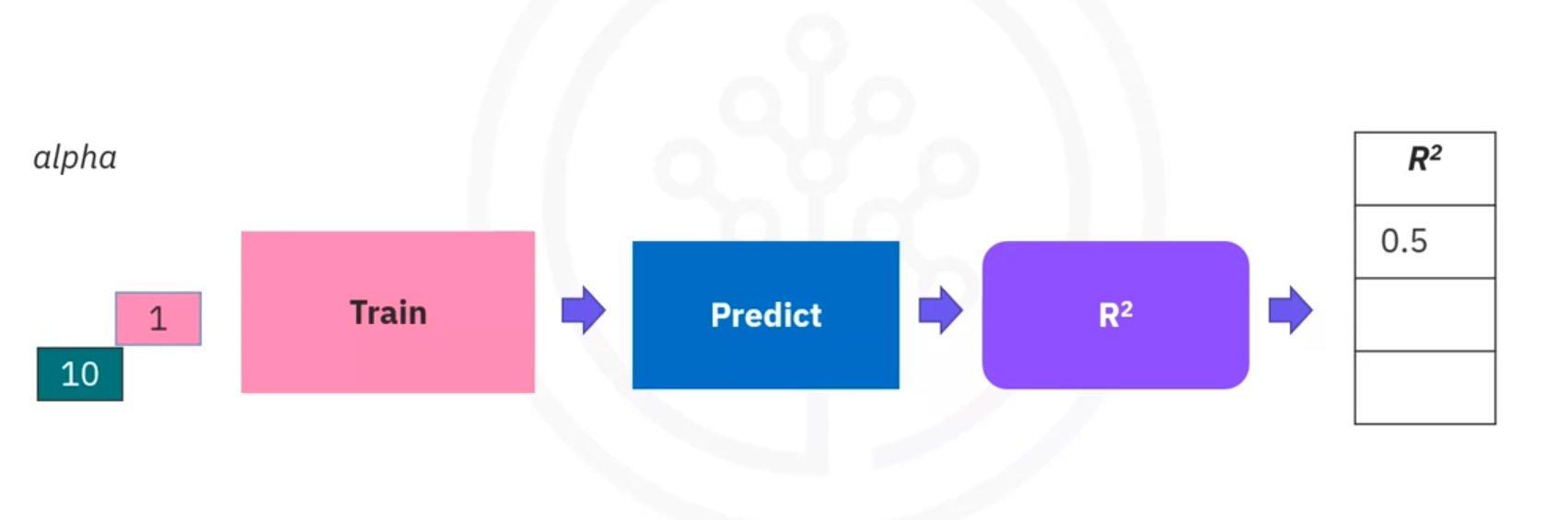
6. Example Visualization:
   • Plot: Shows R^2 values vs. different Alpha values for training and validation data.
   • Interpretation:
     • Training Data: R^2 might increase with Alpha but eventually converge.
     • Validation Data: R^2 may decrease with high Alpha due to reduced model flexibility.

Grid Search for Hyperparameter Tuning

Grid Search

A method for finding the best hyperparameters for a model by systematically evaluating different combinations.

• Hyperparameters: Values like Alpha in Ridge Regression that are not learned from the data but set before the training process.

• Process:
  1. Define Hyperparameters: Set up a grid of hyperparameter values to test. For Ridge Regression, this might include values for Alpha and normalization options.
  2. Train and Evaluate: Train the model using each combination of hyperparameters. Evaluate each model using cross-validation, typically using metrics like R² or Mean Squared Error (MSE).
  3. Select Best Parameters: Choose the hyperparameters that give the best performance based on the evaluation metric.

Implementation in Scikit-learn

import numpy as np
from sklearn.linear_model import Ridge
from sklearn.model_selection import GridSearchCV

# Sample data
X = np.array([[1], [2], [3], [4], [5]])
y = np.array([1, 4, 9, 16, 25])

# Define parameter grid
param_grid = {
    'alpha': [0.1, 1, 10],
    'normalize': [True, False]
}

# Initialize Ridge model
ridge = Ridge()

# Initialize GridSearchCV
grid_search = GridSearchCV(estimator=ridge, param_grid=param_grid, scoring='r2', cv=5)

# Fit GridSearchCV
grid_search.fit(X, y)

# Get best parameters
best_params = grid_search.best_params_
best_score = grid_search.best_score_
best_estimator = grid_search.best_estimator_
cv_results = grid_search.cv_results_

# Results
print("Best Parameters:", best_params)
print("Best Score:", best_score)
print("Best Estimator:", best_estimator)
print("CV Results:", cv_results)

Example Result:

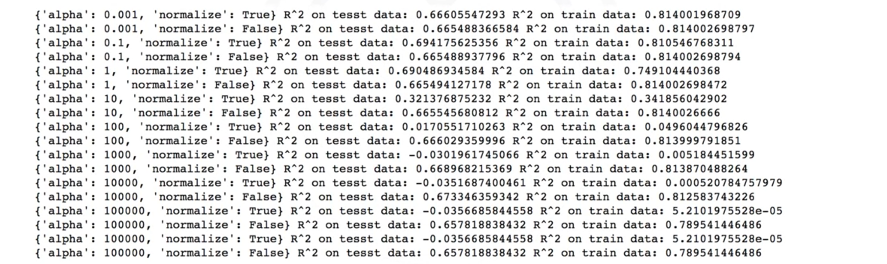
• Key Attributes:
  • best_estimator_: Best model found.
  • cv_results_: Detailed results for each hyperparameter combination, including scores and parameters.

• Advantages: Efficiently explores multiple hyperparameter values to find the best combination, reducing the manual effort required for model tuning.

Cheat Sheet: Model Evaluation and Refinement

Splitting Data for Training and Testing

The process involves separating the target attribute from the rest of the data, treating it as the output, and the rest as input. Then, split these into training and testing subsets.

from sklearn.model_selection import train_test_split

# Define target and features
y_data = df['target_attribute']
x_data = df.drop('target_attribute', axis=1)

# Split into training and testing sets
x_train, x_test, y_train, y_test = train_test_split(x_data, y_data, test_size=0.10, random_state=1)

Cross Validation Score

Cross-validation involves creating multiple subsets of training and testing data to evaluate the model’s performance using the R² value.

from sklearn.model_selection import cross_val_score
from sklearn.linear_model import LinearRegression

# Initialize the model
lre = LinearRegression()

# Perform cross-validation
Rcross = cross_val_score(lre, x_data[['attribute_1']], y_data, cv=n)

# Calculate mean and standard deviation of scores
Mean = Rcross.mean()
Std_dev = Rcross.std()

Cross Validation Prediction

Generate predictions using a cross-validated model.

from sklearn.model_selection import cross_val_predict
from sklearn.linear_model import LinearRegression

# Initialize the model
lre = LinearRegression()

# Perform cross-validation prediction
yhat = cross_val_predict(lre, x_data[['attribute_1']], y_data, cv=4)

Ridge Regression and Prediction

Use Ridge regression to create a model that avoids overfitting by adjusting the alpha parameter and making predictions.

from sklearn.linear_model import Ridge
from sklearn.preprocessing import PolynomialFeatures

# Initialize polynomial features
pr = PolynomialFeatures(degree=2)

# Transform features
x_train_pr = pr.fit_transform(x_train[['attribute_1', 'attribute_2']])
x_test_pr = pr.transform(x_test[['attribute_1', 'attribute_2']])

# Initialize Ridge model
RigeModel = Ridge(alpha=1)

# Fit the model
RigeModel.fit(x_train_pr, y_train)

# Make predictions
yhat = RigeModel.predict(x_test_pr)

Grid Search

Use Grid Search to find the optimal alpha value for Ridge regression by performing cross-validation.

from sklearn.model_selection import GridSearchCV
from sklearn.linear_model import Ridge

# Define parameter grid
parameters = [{'alpha': [0.001, 0.1, 1, 10, 100, 1000, 10000]}]

# Initialize Ridge model
RR = Ridge()

# Initialize GridSearchCV
Grid1 = GridSearchCV(RR, parameters, cv=4)

# Fit GridSearchCV
Grid1.fit(x_data[['attribute_1', 'attribute_2']], y_data)

# Get the best model
BestRR = Grid1.best_estimator_

# Evaluate the model
score = BestRR.score(x_test[['attribute_1', 'attribute_2']], y_test)