Module 2: Artificial Neural Networks

Gradient Descent and Optimization in Neural Networks

Introduction

In this section, we will discuss the concept of gradient descent, a fundamental algorithm used for optimizing weights and biases in neural networks. Understanding gradient descent is crucial before diving into the mechanics of how neural networks learn through backpropagation.

Understanding the Problem

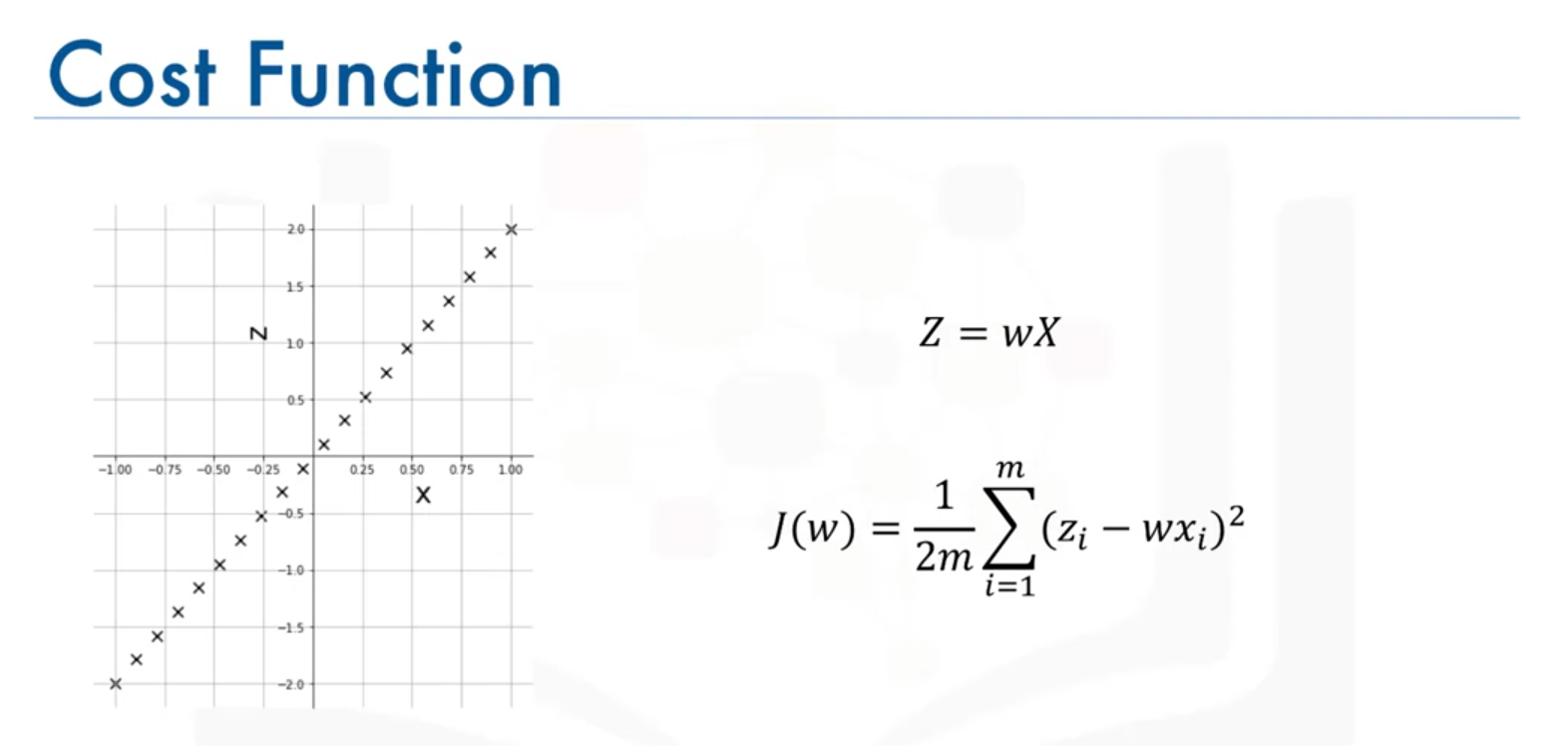
Suppose we have a dataset where $z$ is twice the value of $x$ . Our goal is to find the optimal weight $w$ that generates a line best fitting this data. To achieve this, we define a cost or loss function, denoted as $J$ .

Cost Function

The cost function measures the difference between the actual values of $z$ and the values predicted by the model, i.e., $wx$ . It is given by:

J(w) = \sum_{i=1}^{n} \left( z_i - w \cdot x_i \right)^2

The objective is to find the value of $w$ that minimizes this cost function, leading to the best fit line for the data.

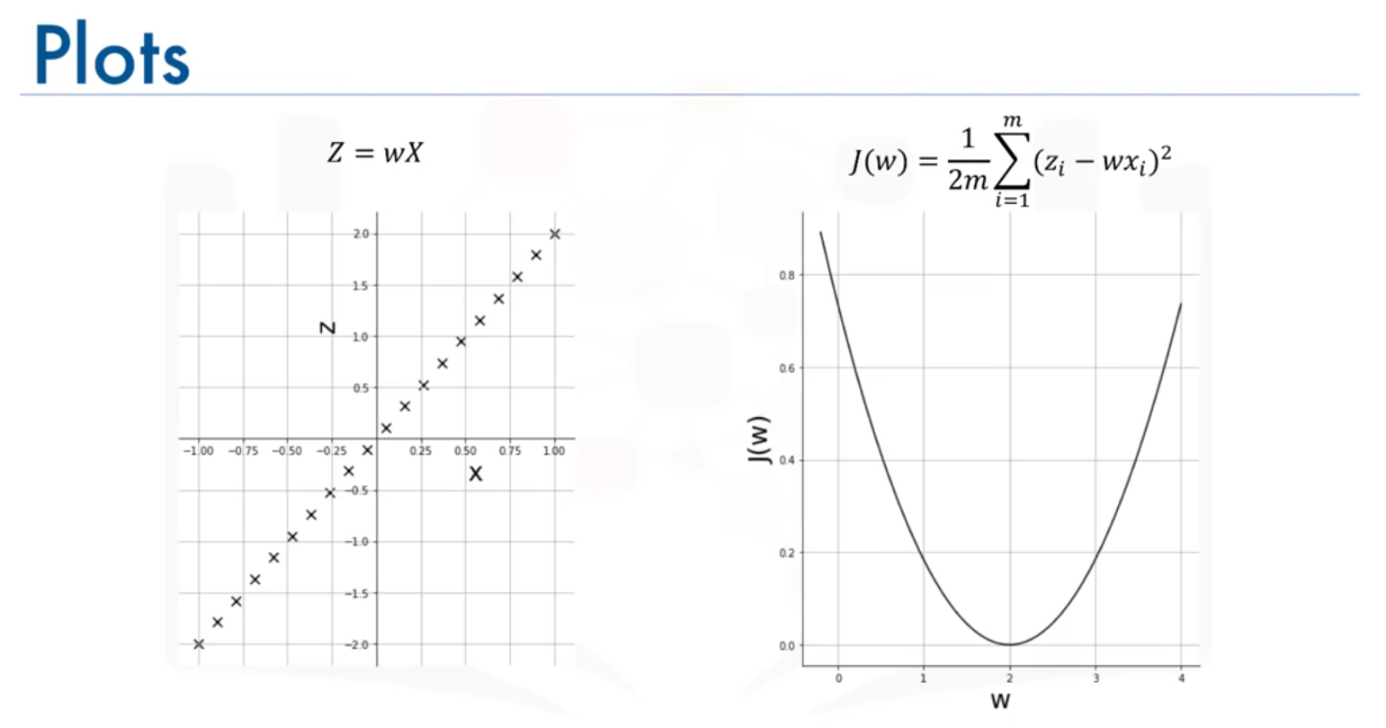
Example: Simple Linear Data

For simplicity, consider the case where $z=2x$ . The optimal value of $w$ that minimizes the cost function is $w=2$ , as it perfectly fits the line $z=2x$ .

Introduction to Gradient Descent

Gradient descent is an iterative optimization algorithm used to find the minimum value of a function. It is particularly useful for minimizing the cost function in neural networks.

How Gradient Descent Works

Initialization: Start with a random initial value of $w$ , denoted as $w_0$ .

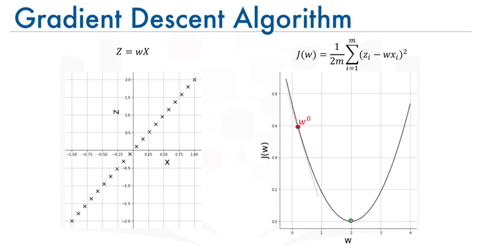
Compute the Gradient: Calculate the gradient (slope OR derivative) of the cost function at the current value of $w$ . The gradient indicates the direction in which the cost function is increasing.

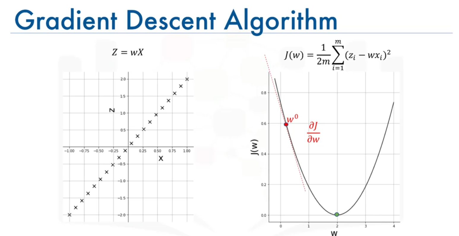
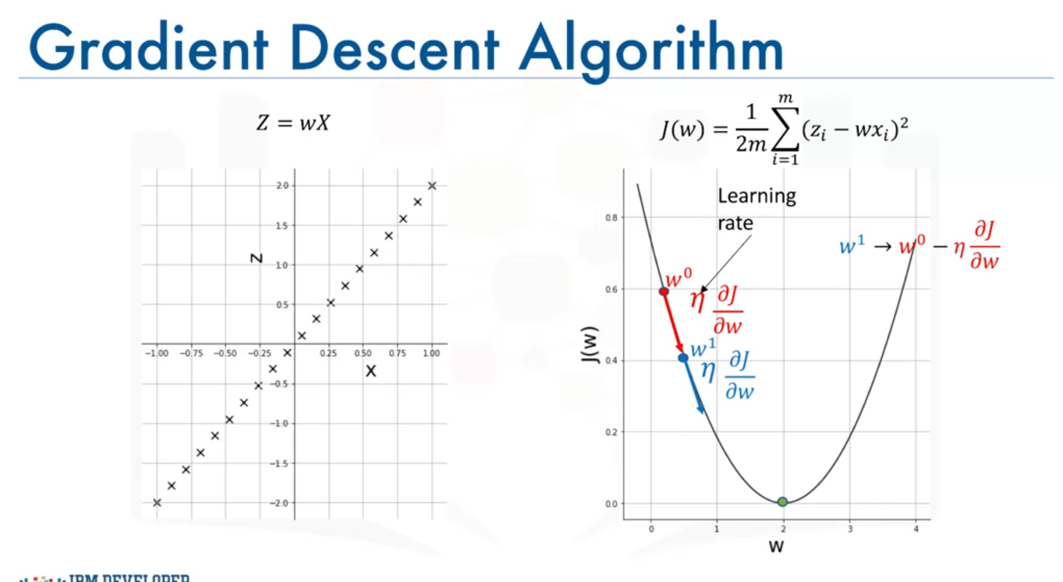
Update Rule: Adjust the value of $w$ by moving in the direction opposite to the gradient. This is done using the formula:

w_{i+1} = w_i - \alpha \cdot \text{gradient}(J(w_i))

Here, $\alpha$ is the learning rate, controlling the step size.

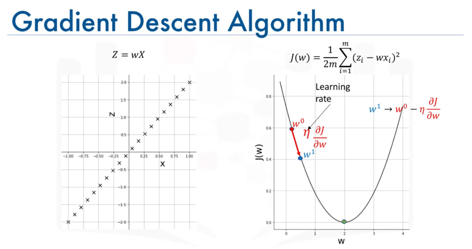
Iteration: Repeat the process until the algorithm converges to the minimum value of the cost function or a value close to it.

Choosing the Learning Rate

Large Learning Rate: Can cause the algorithm to overshoot the minimum, leading to divergence.

Small Learning Rate: Can result in slow convergence, making the algorithm take a long time to reach the minimum.

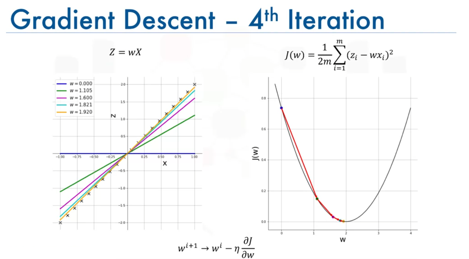
Example with Iterations

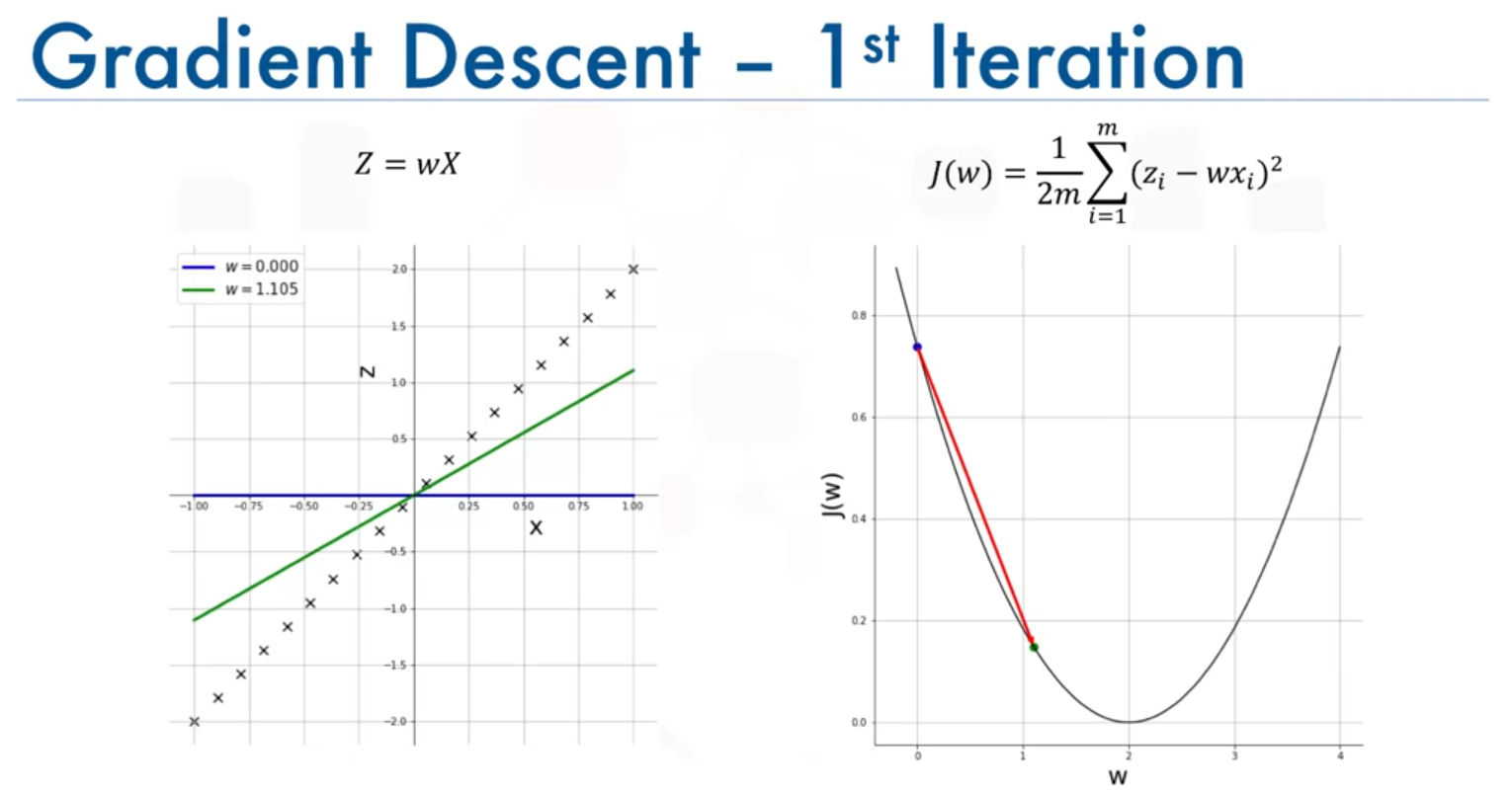
Assume we start with $w_0=0.2$ and use a learning rate $\alpha = 0.4$ :

1st Iteration: $w_1$ moves closer to the optimal value $w=2$ , causing a significant drop in the cost function.

2nd Iteration: $w_2$ continues to move towards $w=2$ , with a smaller step as the slope decreases.

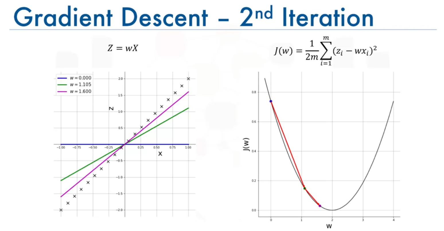
Subsequent Iterations: The steps become smaller as the algorithm approaches the minimum, with the cost function value decreasing steadily.

Application in Neural Networks

In neural networks, gradient descent is used to optimize multiple weights and biases simultaneously. The algorithm updates each parameter in a way that minimizes the overall cost function, which measures how well the network's predictions match the actual data.

Forward Propagation and Gradient Descent

During training, neural networks use forward propagation to calculate the output and then apply gradient descent to adjust the weights and biases, improving the network's performance over time.

Summary

Gradient descent is a powerful optimization algorithm that iteratively adjusts parameters to minimize a cost function. By understanding how to apply gradient descent to a simple linear problem, we are now equipped to explore more complex scenarios, such as optimizing weights in neural networks using backpropagation.

Gradient Descent and Backpropagation in Neural Networks

Training Overview

Neural networks are trained using a supervised learning approach, where each data point has a corresponding label or ground truth. The goal of training is to minimize the difference (error) between the predicted value by the network and the ground truth. This error is calculated and then propagated back into the network to adjust the weights and biases.

Error Calculation and Cost Function

Error (E): The error represents the cost or loss function. It measures how far the network's prediction is from the actual value.

Squared Error: For a single neuron, the error is computed as the squared difference between the predicted value $a_2$ and the ground truth $T$ :
$E = \frac{1}{2} \sum (T - a_2)^2$

In real-world scenarios, the network is trained using large datasets, and the error is calculated as the Mean Squared Error (MSE).

Gradient Descent for Optimization

To minimize the error, gradient descent is used. It iteratively updates the weights and biases in the network:

Starting Point: Begin with random initial weights and biases.

Gradient Calculation: Compute the gradient (slope) of the cost function with respect to each weight and bias using calculus. This shows how much the error will change if we slightly change the weights or biases.

Update Rule: The weights and biases are updated using the formula:

w_{\text{new}} = w_{\text{old}} - \text{learning rate} \times \text{gradient}

The learning rate controls how big a step we take towards the minimum of the cost function.

Backpropagation

Backpropagation is the method used to calculate the gradients of the error with respect to the weights and biases. It applies the chain rule of calculus to compute how the error propagates back through the network:

Derivative Calculation: Derivatives are taken at each layer to determine how the error affects the weights in that layer.

Weight Update: Weights are adjusted by computing the gradient for each weight and applying the gradient descent rule.

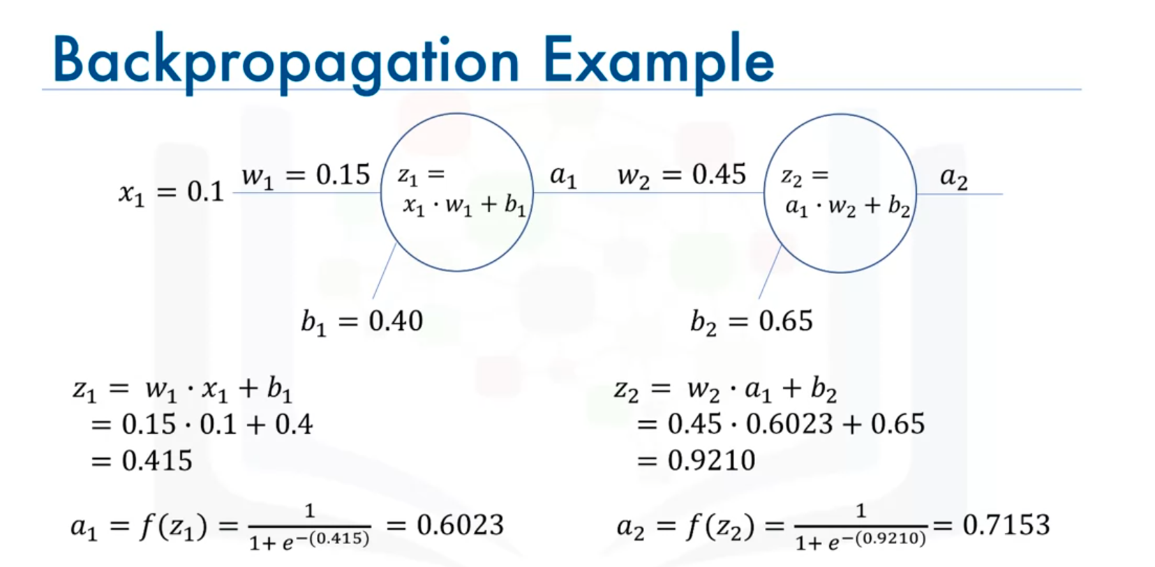
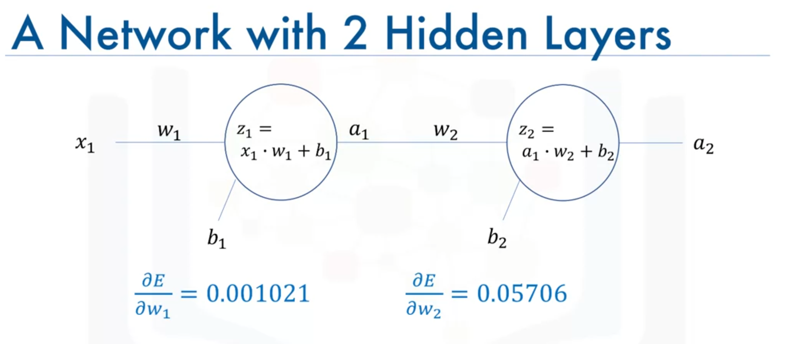
Example with One Input and Two Neurons

Consider a network with two neurons:

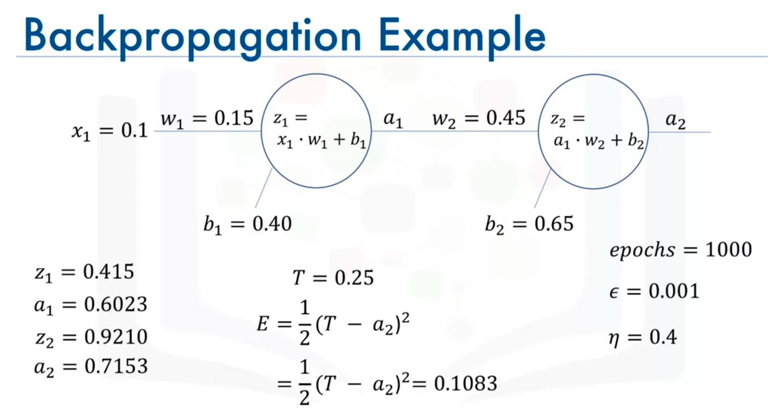
Forward Propagation: Compute the weighted sums $z_1, z_2,$ and the outputs $a_1, a_2$ .

Backpropagation: If the ground truth is known (e.g., 0.25), the error between the prediction and ground truth is calculated. The weights and biases are then updated using the gradients and a learning rate of 0.4.

Weight Update Equations

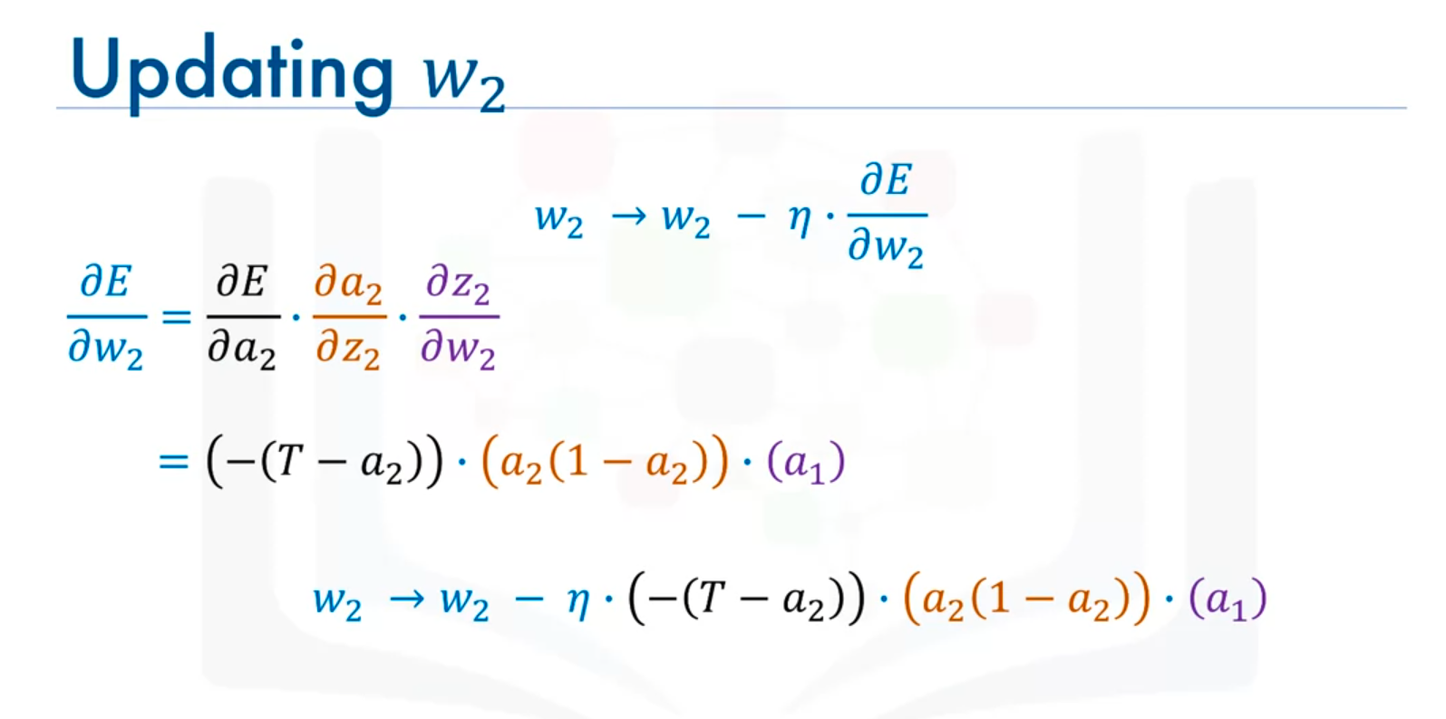
For the second neuron:

Derivative of Error (E) with Respect to Weight $w_2$ :

\frac{\partial E}{\partial w_2} = -(T - a_2) \times a_2 \times (1 - a_2) \times a_1

Update Rule for Weight $w_2$ :
$w_2 = w_2 - \text{learning rate} \times \frac{\partial E}{\partial w_2}$
Similarly, the biases are updated using the derivatives with respect to the biases.
Partial Derivatives Document

Iterative Training Process

Training involves repeatedly performing the following steps until the error is minimized:

Forward Propagation: Calculate the network output.

Error Calculation: Compute the error between the prediction and ground truth.

Backpropagation: Calculate gradients for each weight and bias using the chain rule.

Update Weights and Biases: Adjust parameters to reduce the error.

This process continues over multiple iterations or epochs until the error is sufficiently small or the maximum number of iterations is reached.

Vanishing Gradient Problem in Neural Networks

Overview

The vanishing gradient problem is a significant issue associated with using the sigmoid activation function in neural networks. It affects the training efficiency and prediction accuracy of the network.

Problem Description

Sigmoid Activation Function: The sigmoid function maps input values to a range between 0 and 1. While this can be useful, it leads to problems during backpropagation.

Gradients in Backpropagation: During backpropagation, the gradients of the error with respect to the weights are computed. For the sigmoid function, the gradient (derivative) of the activation function is always between 0 and 1. This causes the gradients to become very small as they are propagated backward through the network.

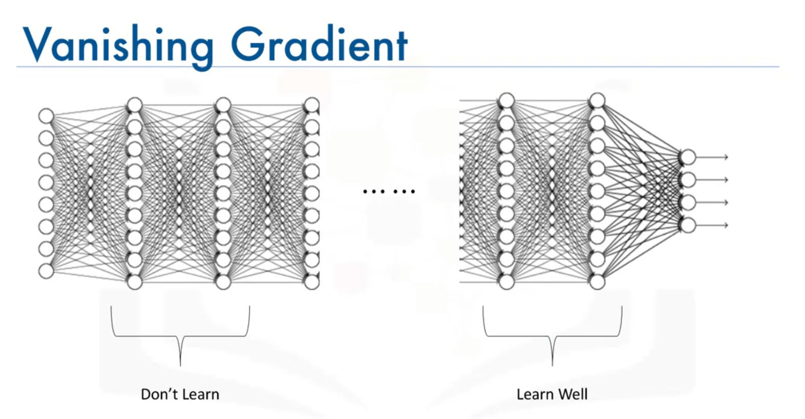
Effect on Learning: In a neural network with multiple layers, gradients of weights in earlier layers become very small. This results in:
- Slow Learning: Neurons in earlier layers learn very slowly compared to neurons in later layers.
- Long Training Time: Training takes significantly longer.
- Compromised Accuracy: The prediction accuracy of the network may be affected due to inefficient learning in earlier layers.

Mathematical Insight

When using the sigmoid function, the derivatives of the activation function can be very small. During backpropagation, the gradient of the error with respect to the weights is calculated as a product of these derivatives. Thus, gradients tend to diminish as they propagate backward through the network:

\text{Gradient} = \frac{\partial E}{\partial w_i} = \frac{\partial E}{\partial a_n} \cdot \frac{\partial a_n}{\partial z_n} \cdot \frac{\partial z_n}{\partial w_i}

where:

$\frac{\partial E}{\partial a_n}$ is the gradient of the error with respect to the output $a_n$ .

$\frac{\partial a_n}{\partial z_n}$ is the gradient of the sigmoid function, which is small.

$\frac{\partial z_n}{\partial w_i}$ depends on the inputs.

Conclusion

Due to the vanishing gradient problem, sigmoid functions and similar activation functions are not ideal for deep networks. This problem has led to the development and use of alternative activation functions that mitigate this issue.

Next Steps

In the following notes, alternative activation functions that address the vanishing gradient problem will be introduced. These functions are commonly used in hidden layers of modern neural networks to improve training efficiency and accuracy.

Activation Functions in Neural Networks

Types of Activation Functions

There are 7 types of most common activation functions:

Sigmoid Function

Hyperbolic Tangent (tanh) Function

Rectified Linear Unit (ReLU) Function

Softmax Function

Binary Step Function

Linear Function

Leaky ReLU

Additional Note: 5-6-7 are not popular functions.

Introduction

Activation functions are crucial for the learning process of neural networks. They introduce non-linearity into the model, allowing it to learn complex patterns. While the sigmoid function was commonly used in the past, it has notable shortcomings, such as the vanishing gradient problem. This note explores several activation functions and their applications.

1. Sigmoid Function

Formula

\sigma(z) = \frac{1}{1 + e^{-z}}

Range

(0, 1)

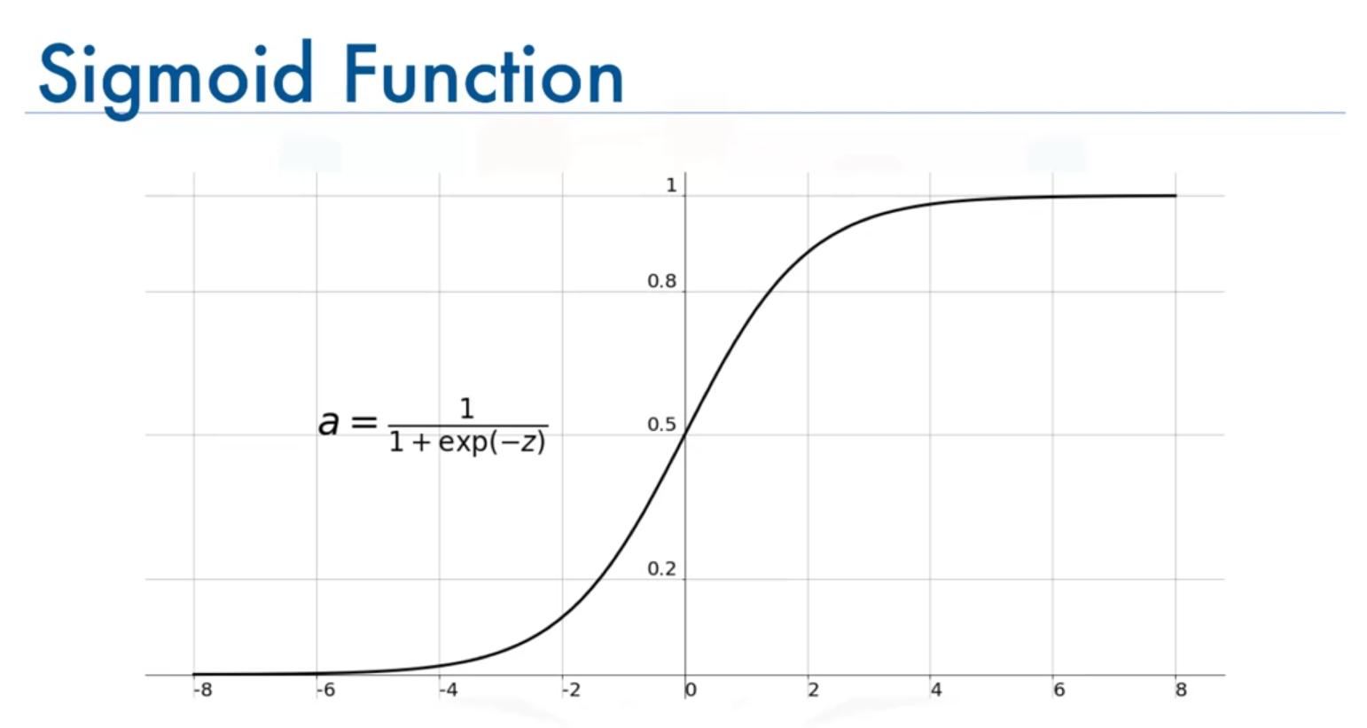
Characteristics

Outputs values between 0 and 1.

Gradients become very small in the regions where $z$ is very large or very small, leading to the vanishing gradient problem.

Not symmetric around the origin; all outputs are positive.

Applications

Previously popular, but avoided in deep networks due to vanishing gradients.

2. Hyperbolic Tangent (tanh) Function

Formula

\tanh(z) = \frac{e^z - e^{-z}}{e^z + e^{-z}}

Range

(-1, 1)

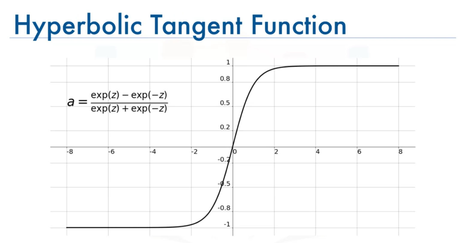
Characteristics

Similar to the sigmoid function but symmetric around the origin.

Gradients can still become very small in deep networks, leading to the vanishing gradient problem.

Applications

Used in some applications but also limited by vanishing gradients in very deep networks.

3. Rectified Linear Unit (ReLU) Function

Formula

\text{ReLU}(z) = \max(0, z)

Range

[ 0, \infty)

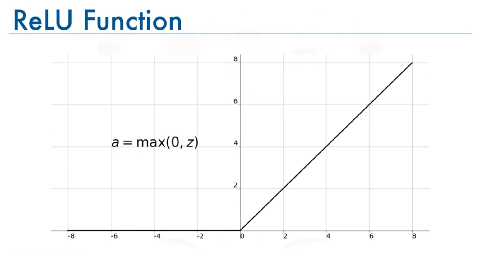
Characteristics

Non-linear activation function that only activates neurons with positive input values.

Helps overcome the vanishing gradient problem by ensuring that gradients are not zero for positive inputs.

Results in sparse activation where only a few neurons are activated at a time.

Applications

Widely used in hidden layers of deep networks due to its efficiency and effectiveness.

4. Softmax Function

Formula

\text{Softmax}(z_i) = \frac{e^{z_i}}{\sum_{j} e^{z_j}}

Range

(0, 1) \text{ (sums to 1 across the output layer)}

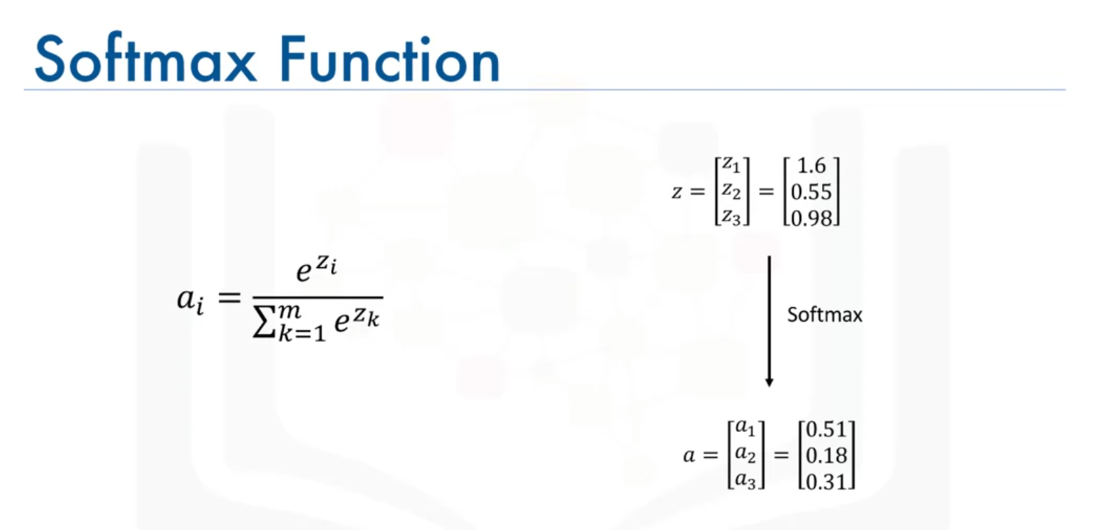
Characteristics

Converts raw output scores into probabilities that sum to 1.

Useful for classification tasks where we need to determine the probability of each class.

Applications

Commonly used in the output layer of classification networks to handle multi-class problems..

Conclusion

Sigmoid and tanh Functions: Avoided in many modern applications due to the vanishing gradient problem.

ReLU Function: Preferred activation function in hidden layers of deep networks due to its effectiveness and ability to mitigate vanishing gradients.

Softmax Function: Useful for classification tasks to provide class probabilities.

This concludes the overview of activation functions. For deep learning applications, start with ReLU and consider other functions if necessary based on performance.