Deep Neural Networks: An Introduction

Overview

Neural networks have evolved significantly over time, transitioning from shallow networks to deep neural networks (DNNs) that handle complex tasks and data types. This note explores the distinctions between shallow and deep neural networks, and the reasons behind the recent advancements in deep learning.

Shallow vs. Deep Neural Networks

Shallow Neural Networks

• Definition: A shallow neural network typically has only one hidden layer.

• Characteristics:
  • Simpler architectures
  • Limited ability to extract features from raw data
  • Often used for simpler tasks or as building blocks for deeper networks

Deep Neural Networks

• Definition: A deep neural network has multiple hidden layers and neurons.

• Characteristics:
  • Capable of learning hierarchical features from raw data such as images and text
  • Ability to extract features from raw data.
  • Handles more complex tasks and datasets
  • Example: Image recognition, natural language processing

Factors Contributing to the Rise of Deep Learning

1. Advancements in Neural Network Techniques

• ReLU Activation Function:
  • Addressed the vanishing gradient problem
  • Enabled the training of very deep networks

2. Availability of Data

• Importance:
  • Deep neural networks excel with large datasets
  • Large data helps prevent overfitting

• Current Trends:
  • Access to vast amounts of data has become easier
  • Deep learning algorithms benefit significantly from increased data

3. Computational Power

• GPU Utilization:
  • NVIDIA GPUs and other high-performance computing resources
  • Reduced training times from weeks to hours

• Impact:
  • Enables experimentation with different network architectures and prototypes in shorter periods

Conclusion

The combination of advancements in neural network techniques, the availability of large datasets, and increased computational power has driven the recent boom in deep learning. The field continues to evolve, with deep neural networks becoming increasingly prevalent in various applications. Upcoming topics will delve into supervised deep learning algorithms and convolutional neural networks (CNNs).

Introduction to Convolutional Neural Networks (CNNs) (Supervised Deep Learning Model)

Overview

Convolutional Neural Networks (CNNs) are a specialized type of neural network designed for processing structured grid data such as images. This note covers the fundamental architecture of CNNs, their operational mechanisms, and how to build them using the Keras library.

Convolutional Neural Networks (CNNs)

Architecture

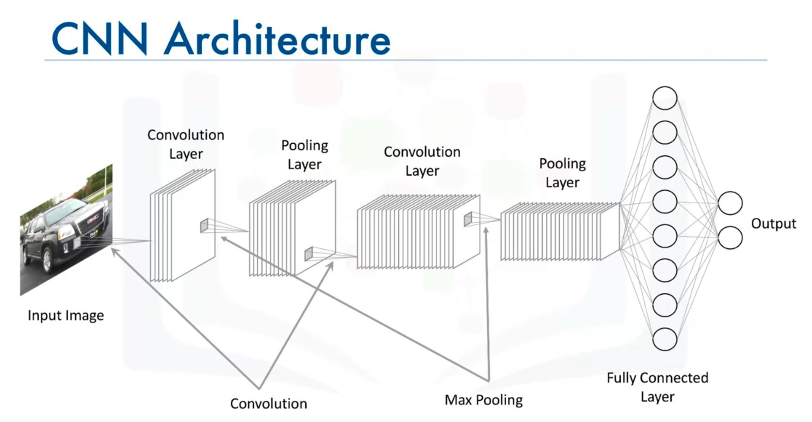
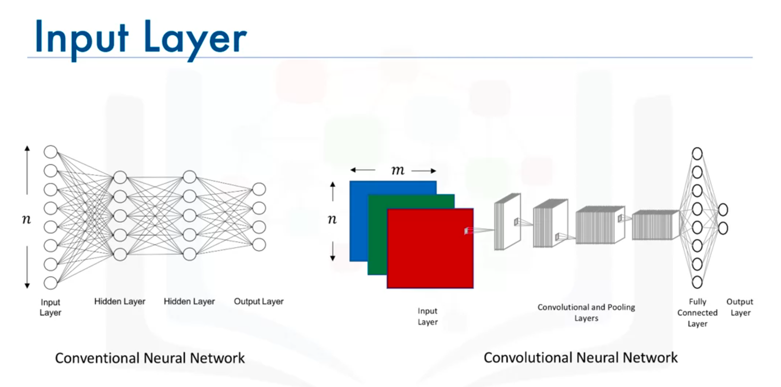
Image Input Dimensions

• Grayscale Images: (n x m x 1)

• Colored Images: (n x m x 3), where 3 represents RGB channels.

Key Components of CNNs

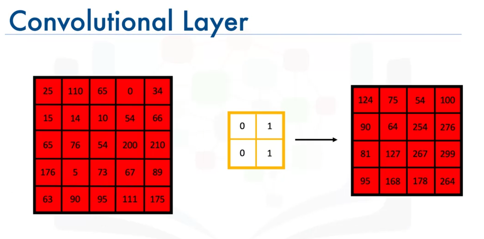
1. Convolutional Layer

• Purpose: Applies filters to the input image to produce feature maps.

• Filter: A small matrix used to detect features such as edges, textures, or patterns.

• Operation: Computes the convolution operation between the filter and the input image.
  • Filter Size: e.g., (2 x 2)
  • Stride: The number of pixels by which the filter moves across the image.
  • Output: An empty matrix filled with results from the convolution process

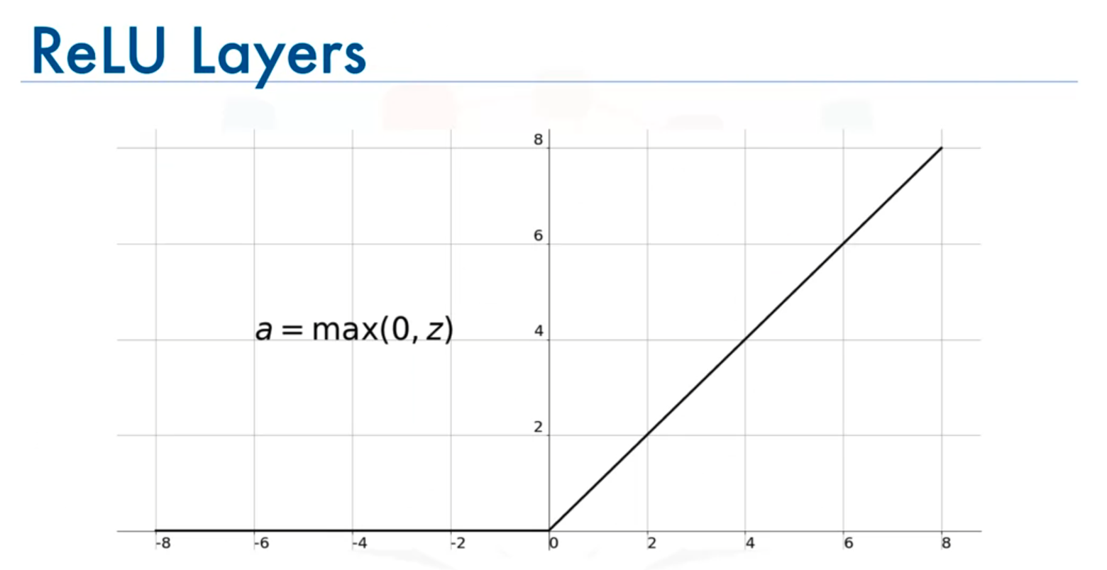
2. Activation Function (ReLU)

• Purpose: Introduces non-linearity into the model.

• Operation: Applies the ReLU (Rectified Linear Unit) function to the output of the convolutional layer.
  • ReLU Function: Outputs the input directly if it is positive; otherwise, it outputs zero.

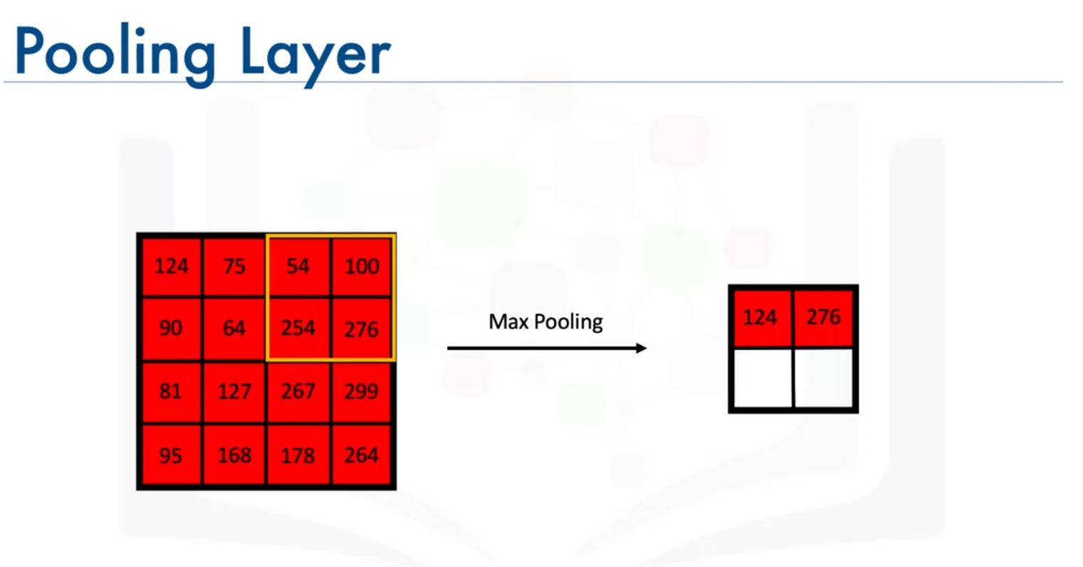
3. Pooling Layer

• Purpose: Reduces the spatial dimensions of the feature maps.

• Types:
  • Max-Pooling: Selects the maximum value from each section of the feature map.
    • Filter Size: e.g., (2 x 2)
    • Stride: The number of pixels by which the pooling filter moves.
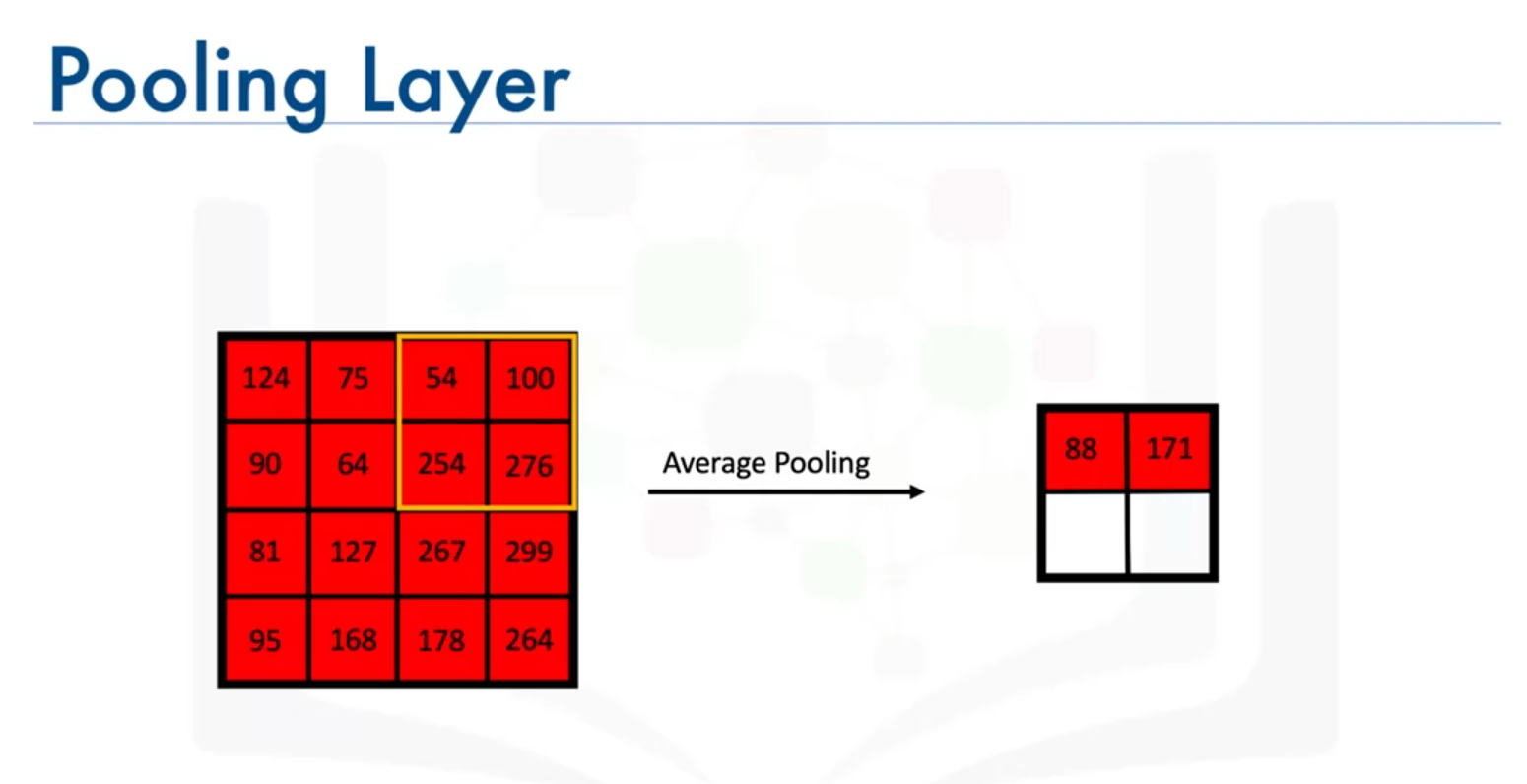
  • Average-Pooling: Computes the average value from each section of the feature map.

• Benefit: Reduces computational complexity and helps prevent overfitting.

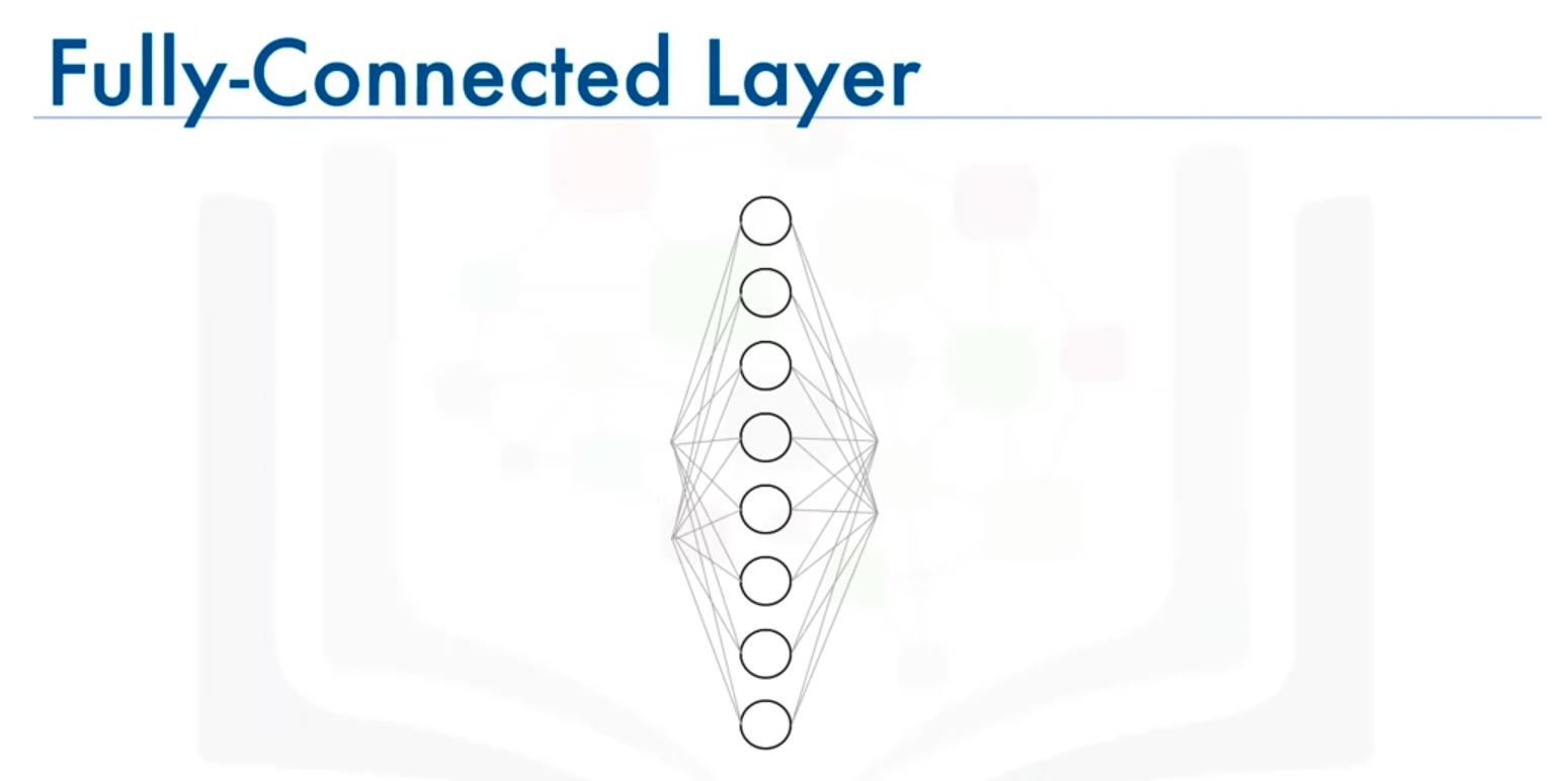
4. Fully Connected Layer

• Purpose: Connects every node from the previous layer to every node in the current layer.

• Operation: Flattens the output from the previous layers and produces an n-dimensional vector, where n corresponds to the number of classes.

• Activation Function: Typically uses the softmax function to convert the outputs into probabilities.

CNN Architecture

• Input Layer: Defines the size of the input images (e.g., 128 x 128 x 3 for color images).

• Convolutional Layers: Apply multiple filters and include ReLU activation.

• Pooling Layers: Apply max-pooling or average-pooling.

• Fully Connected Layers: Flatten the data and produce output based on the number of classes.

• Output Layer: Produces the final class probabilities using the softmax activation function.

Summary

• Efficiency: CNNs reduce the number of parameters compared to traditional neural networks, making them computationally efficient.

• Applications: Ideal for tasks involving image recognition, object detection, and other computer vision problems.

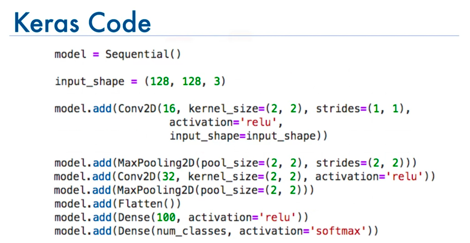
Building CNNs with Keras

1. Model Creation:
   • Use the Sequential model to build the CNN.

2. Defining Input Shape:
   • For 128x128 color images: input_shape=(128, 128, 3)

3. Adding Layers:
   • Convolutional Layer:

     model.add(Conv2D(16, (2, 2), strides=(1, 1), activation='relu', input_shape=(128, 128, 3)))

     • Parameters:
       • 16: Number of filters or kernels.
       • (2, 2): Size of each filter.
       • strides=(1, 1): The step size with which the filter moves across the image.
       • activation='relu': Activation function applied after the convolution operation.
       • input_shape=(128, 128, 3): Shape of the input images. For color images, the last dimension is 3 (RGB channels).
   • Pooling Layer:

     model.add(MaxPooling2D(pool_size=(2, 2), strides=(2, 2)))

     • Parameters:
       • pool_size=(2, 2): Size of the pooling window.
       • strides=(2, 2): The step size with which the pooling window moves across the image.
   • Additional Convolutional and Pooling Layers:

     model.add(Conv2D(32, (2, 2), strides=(1, 1), activation='relu'))
     model.add(MaxPooling2D(pool_size=(2, 2), strides=(2, 2)))

     • Parameters:
       • 32: Number of filters or kernels in this convolutional layer.
       • (2, 2): Size of each filter.
       • strides=(1, 1): The step size with which the filter moves across the image.
       • activation='relu': Activation function applied after the convolution operation.
       • pool_size=(2, 2): Size of the pooling window.
       • strides=(2, 2): The step size with which the pooling window moves across the image.

4. Flattening and Fully Connected Layers:
   • Flatten: Converts 3D feature maps into 1D.

     model.add(Flatten())

   • Dense Layers:

     model.add(Dense(100, activation='relu'))
     model.add(Dense(num_classes, activation='softmax'))

     • Parameters:
       • 100: Number of neurons in the dense layer.
       • activation='relu': Activation function applied to the neurons in the dense layer.
       • num_classes: Number of output neurons, typically equal to the number of classes in the classification problem.
       • activation='softmax': Activation function applied to the output layer to convert raw scores into probabilities.

5. Compilation:
   • Define optimizer, loss function, and metrics:

     model.compile(optimizer='adam', loss='categorical_crossentropy', metrics=['accuracy'])

     • Parameters:
       • optimizer='adam': Optimization algorithm used for training.
       • loss='categorical_crossentropy': Loss function used for classification tasks with multiple classes.
       • metrics=['accuracy']: Evaluation metric used to measure the performance of the model.

6. Training and Validation:
   • Train the model using the fit method and validate using a test set.

Conclusion

CNNs are powerful for image processing tasks due to their ability to automatically extract and learn features from images. The architecture involves convolutional, activation, pooling, and fully connected layers, which collectively enable the network to perform tasks such as image recognition and object detection.

Recurrent Neural Networks (RNNs) Overview (Unsupervised Deep Learning Model)

Introduction to RNNs

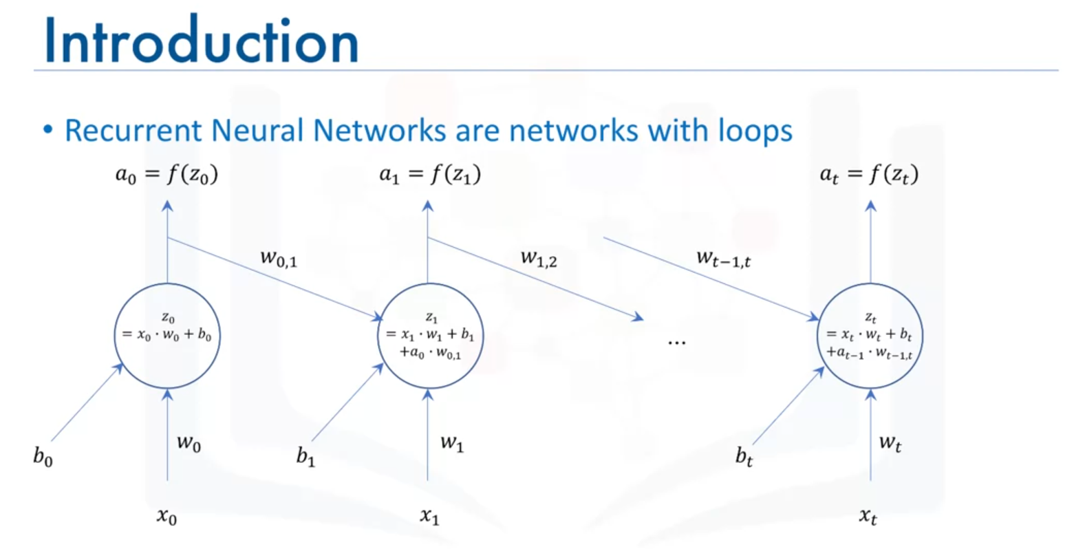
• Purpose: RNNs are used to analyze sequences where data points are not independent but rather follow a temporal or sequential relationship.

• Architecture: RNNs include loops that allow them to take both the current input and the output from the previous data point into account.

How RNNs Work

• Input and Output at Each Time Step:
  • At time t = 0, the network takes in input $x_0$ and outputs $a_0$.
  • At time t = 1, the network takes in input $x_1$ and the previous output $a_0$, weighted by $w_{1,2}$.
  • This process continues, incorporating previous outputs into the computation at each step.

Applications of RNNs

• Text Analysis: Suitable for processing and modeling sequential text data.

• Genomic Data: Can analyze sequences in genetic information.

• Handwriting: Applied in handwriting generation and recognition.

• Stock Markets: Used for predicting stock prices based on historical data.

Long Short-Term Memory (LSTM) Networks

• Overview: A specialized type of RNN designed to overcome some limitations of traditional RNNs.

• Applications:
  • Image Generation: Models trained on images to generate novel images.
  • Handwriting Generation: Creating handwritten text based on trained models.
  • Image Description: Automatically describing images.
  • Video Streams: Analyzing and describing video sequences.

Summary

• RNNs: Effective for tasks involving sequences and temporal data.

• LSTM Models: A specific type of RNN that handles long-term dependencies and is used in advanced applications like image and video analysis.

Autoencoders and Restricted Boltzmann Machines (RBMs)

Introduction to Autoencoders

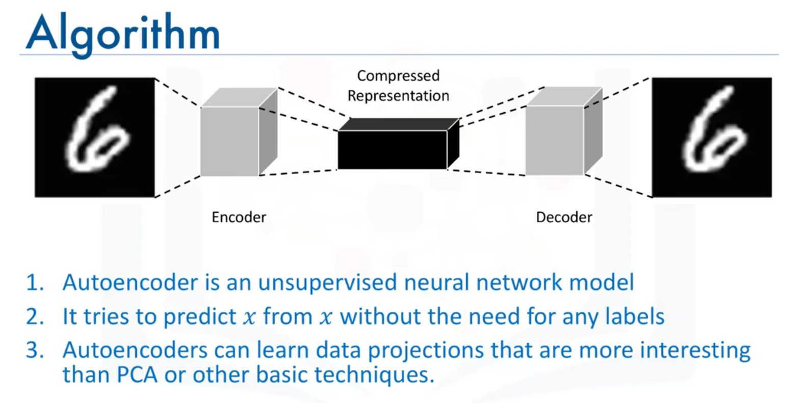
• Definition: Autoencoders are unsupervised deep learning models used for data compression. They learn to compress and decompress data automatically through neural networks.

• Purpose: They aim to learn a compressed representation of the input data and then reconstruct the original data from this representation.

• Training: Autoencoders use backpropagation with the target variable being the same as the input, effectively learning an approximation of an identity function.

Architecture of an Autoencoder

• Encoder:
  • Compresses the input data into a lower-dimensional representation.

• Decoder:
  • Reconstructs the original data from the compressed representation.

Applications of Autoencoders

• Data Denoising: Removing noise from data to recover the original signal.

• Dimensionality Reduction: Reducing the number of features in the data for visualization purposes.

Advantages over Traditional Methods

• Non-Linear Transformations: Autoencoders, with their non-linear activation functions, can learn more complex projections compared to linear methods like Principal Component Analysis (PCA).

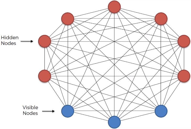
Restricted Boltzmann Machines (RBMs)

• Overview: RBMs are a type of autoencoder that can learn the distribution of the input data to perform tasks such as:
  • Fixing Imbalanced Datasets: Generating more data points for minority classes to balance datasets.
  • Estimating Missing Values: Predicting missing feature values in datasets.
  • Automatic Feature Extraction: Learning features from unstructured data.

Summary

• Autoencoders: Useful for data compression, denoising, and dimensionality reduction.

• RBMs: Specialized autoencoders effective for handling imbalanced datasets, estimating missing values, and feature extraction.

This concludes the introduction to autoencoders and Restricted Boltzmann Machines (RBMs).