Introduction to Regression

Overview

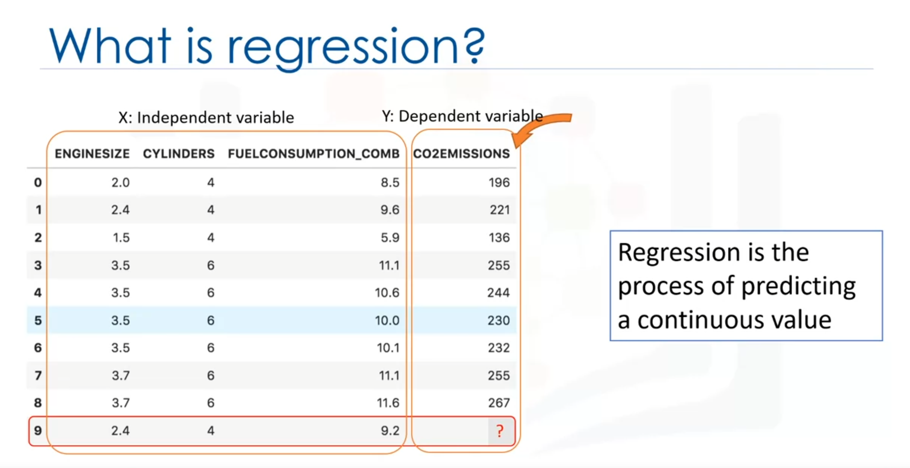
Regression is the process of predicting a continuous value using other variables. It involves two types of variables: dependent (target) and independent (explanatory) variables. The dependent variable is the value being predicted, while the independent variables are the factors used to make the prediction. In regression, the dependent variable should be continuous, whereas the independent variables can be either categorical or continuous.

Example Dataset

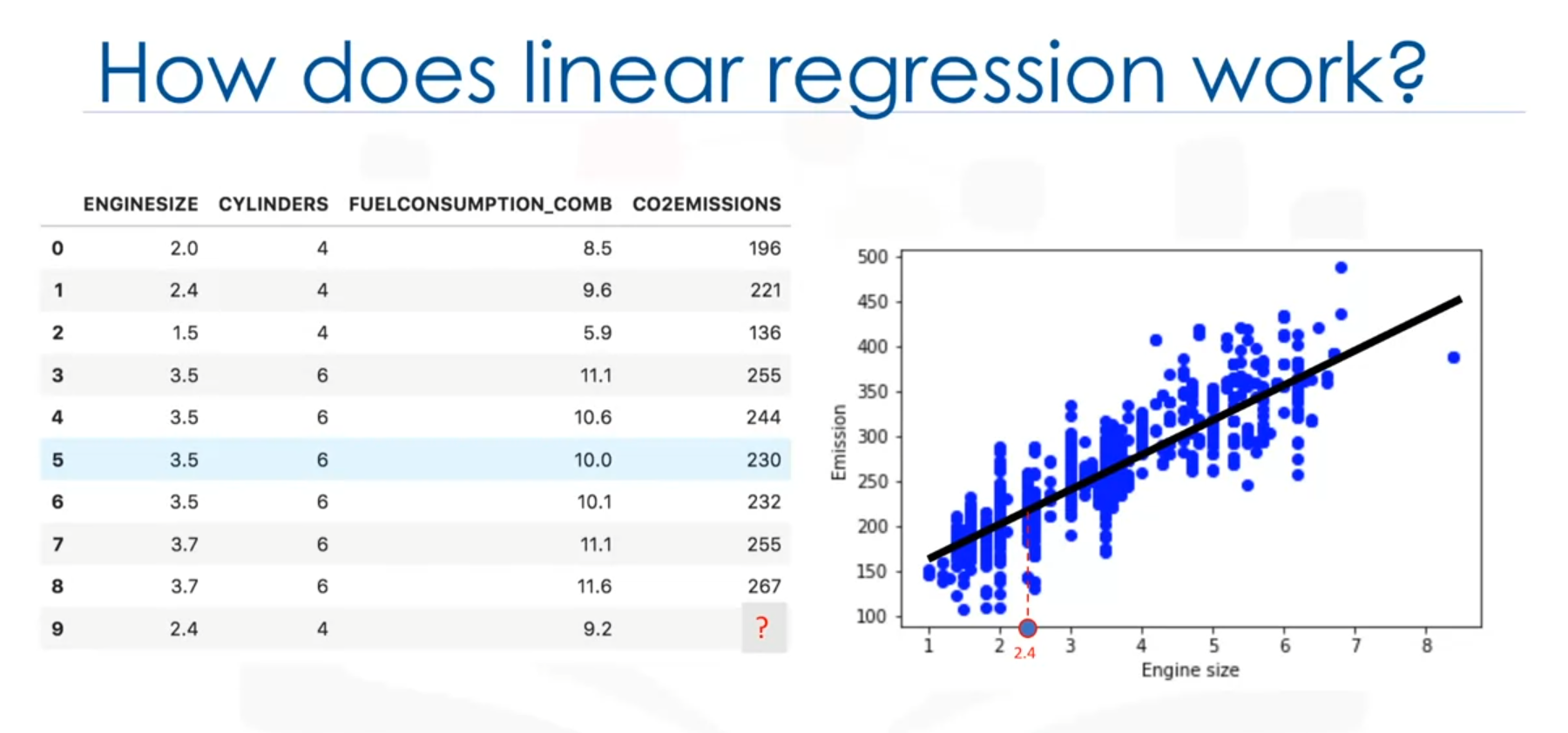
Consider a dataset related to CO2 emissions from different cars. The dataset includes:

• Engine size

• Number of cylinders

• Fuel consumption

• CO2 emission

Predictive Question

Given this dataset, is it possible to predict the CO2 emission of a car using other fields such as engine size or cylinders? → Yes

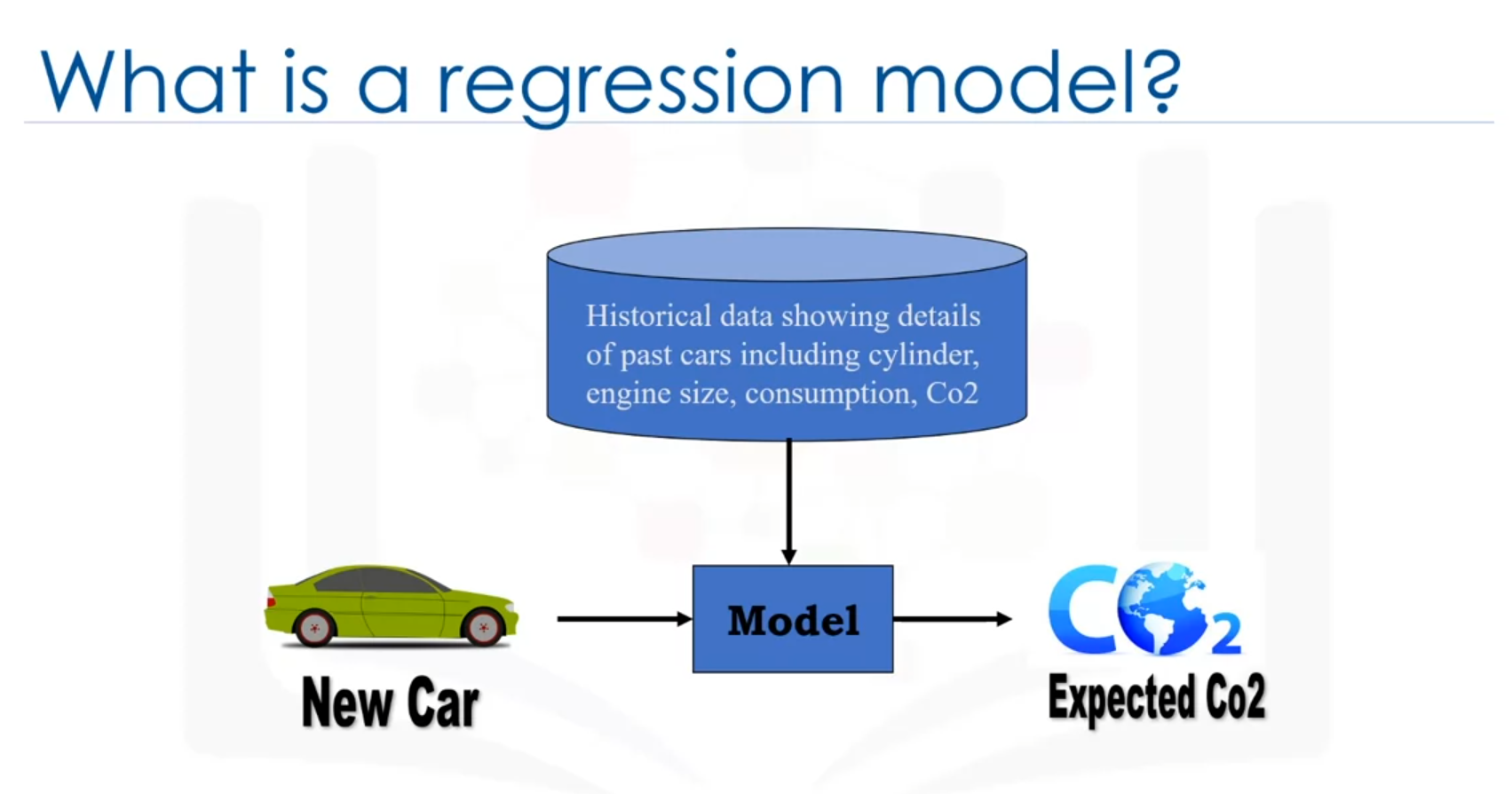
Historical Data and Prediction

Assume there is historical data from different cars. The goal is to estimate the CO2 emission of a new or unknown car, such as the one in row 9, which hasn't been manufactured yet. Regression methods can be used to make this prediction.

Types of Variables in Regression

• Dependent Variable (Y): The state, target, or final goal to be predicted.

• Independent Variables (X): The causes or explanatory variables.

Types of Regression Models

Simple Regression

• Definition: Uses one independent variable to estimate a dependent variable.

• Example: Predicting CO2 emission using the variable of engine size.

• Nature: Can be linear or non-linear based on the relationship between the independent and dependent variables.

Multiple Regression

• Definition: Uses more than one independent variable to estimate a dependent variable.

• Example: Predicting CO2 emission using engine size and the number of cylinders.

• Nature: Can be linear or non-linear depending on the relationship between the dependent and independent variables.

Applications of Regression

Sales Forecasting

Predicting a salesperson's total yearly sales using independent variables such as age, education, and years of experience.

Psychology

Determining individual satisfaction based on demographic and psychological factors.

Real Estate

Predicting the price of a house based on its size, number of bedrooms, and other features.

Employment Income

Predicting employment income using variables such as hours of work, education, occupation, age, and years of experience.

Other Fields

Regression analysis is also useful in finance, healthcare, retail, and more.

Conclusion

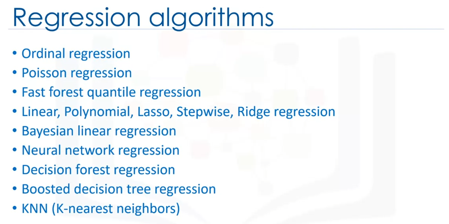
Regression analysis has numerous applications across various fields. It helps in estimating continuous values using historical data and independent variables. Various regression algorithms exist, each suited to specific conditions, providing a foundation for exploring different regression techniques.

Introduction to Linear Regression

Linear regression is an effective method for predicting a continuous value using other variables. This introduction provides the necessary background to use linear regression effectively.

Dataset Overview

Consider a dataset related to CO2 emissions of different cars. The dataset includes:

• Engine size

• Number of cylinders

• Fuel consumption

• CO2 emissions

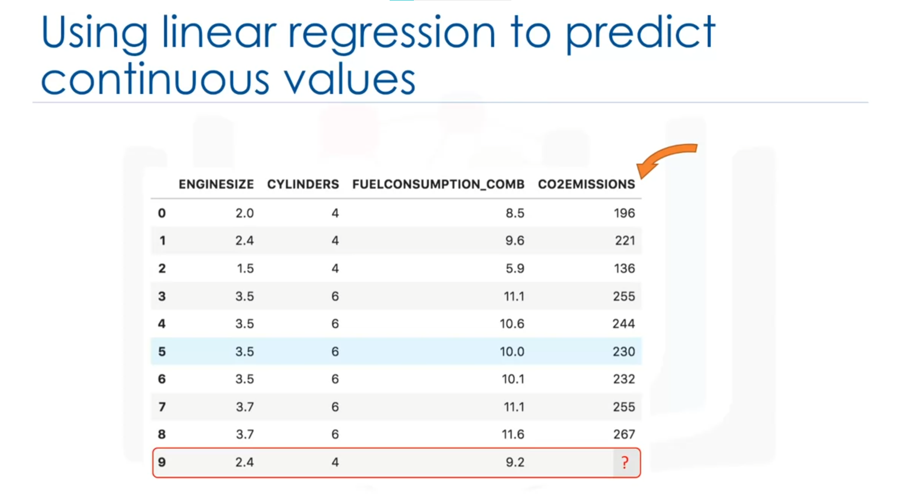
The goal is to predict the CO2 emission of a car using another field, such as engine size. Linear regression can be used for this purpose.

Linear Regression Basics

Linear regression is the approximation of a linear model to describe the relationship between two or more variables.

Variables in Linear Regression

• Dependent Variable (Y): The continuous value being predicted.

• Independent Variable (X): The explanatory variable(s), which can be categorical or continuous.

Types of Linear Regression

1. Simple Linear Regression:
   • Uses one independent variable to estimate a dependent variable.
   • Example: Predicting CO2 emission using engine size.

2. Multiple Linear Regression:
   • Uses more than one independent variable to estimate a dependent variable.
   • Example: Predicting CO2 emission using engine size and number of cylinders.

How Linear Regression Works

Scatter Plot

A scatter plot can be used to visualize the relationship between variables, such as engine size (independent variable) and CO2 emission (dependent variable). The plot helps to identify if the variables are linearly related.

Fitting a Line

Linear regression fits a line through the data points. For example, as the engine size increases, the CO2 emissions also increase. The objective is to find a line that best fits the data, which can be used to predict CO2 emissions.

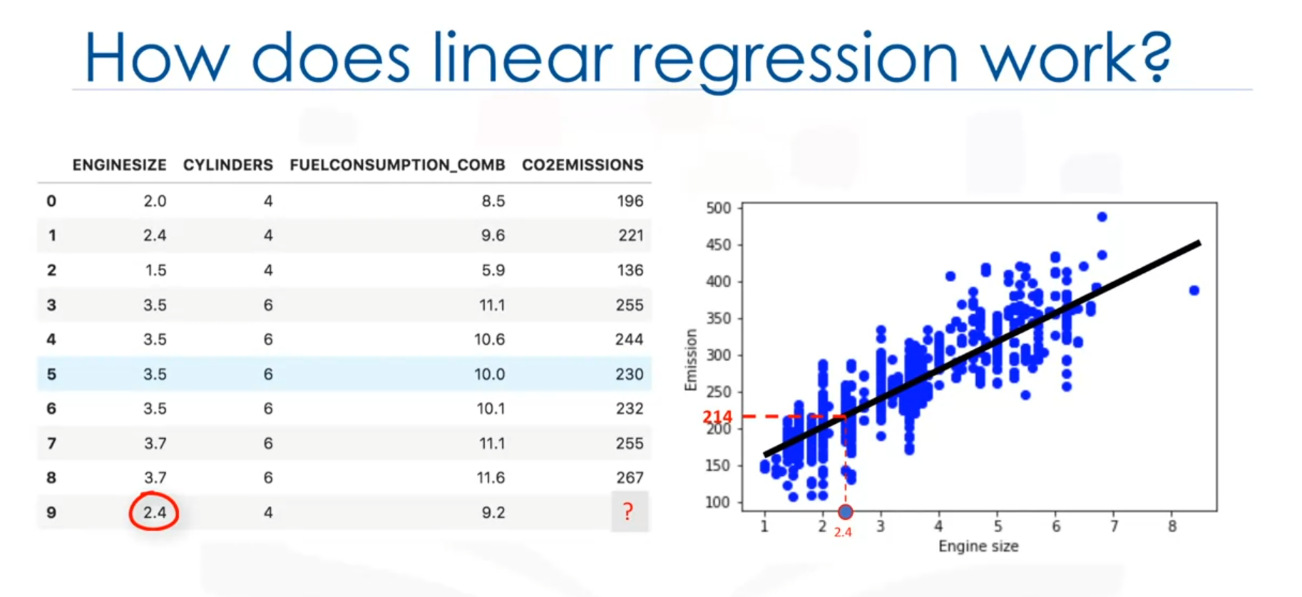
Prediction Using the Line

Assuming the line is a good fit, it can be used to predict the CO2 emission of an unknown car. For example, for a car with an engine size of 2.4, the predicted CO2 emission is 214.

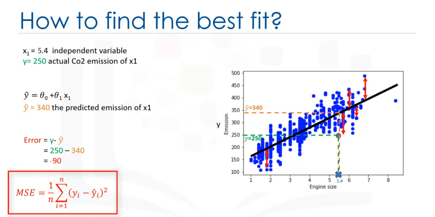
Mathematical Representation

The fitted line in linear regression is represented as a polynomial. For a simple linear regression with one independent variable , the model is:

$\hat{y} = \theta_0 + \theta_1 x_1$

• $\hat{y}$: Predicted value (dependent variable)

• $x_1$: Independent variable

• $\theta_0$: Intercept

• $\theta_1$: Slope or gradient of the line

Estimating Coefficients

• $\theta_0$ (intercept) and $θ_1$ (slope) are the parameters of the line that need to be adjusted to minimize the error.

• The goal is to minimize the mean squared error (MSE), which is the mean of all residual errors (the distance from data points to the fitted line).

Calculating $θ_0$ and $θ_1$

1. Calculate the Mean:
   • Calculate the mean of the independent variable ($\bar{x}$) and the dependent variable ($\hat{y}$).

2. Estimate $θ_1$ (slope):

   $$\theta_1 = \frac{\sum (x_i - \bar{x})(y_i - \bar{y})}{\sum (x_i - \bar{x})^2}$$

3. Estimate $\theta_0$ (intercept):

   $$\theta_0 = \bar{y} - \theta_1 \bar{x}$$

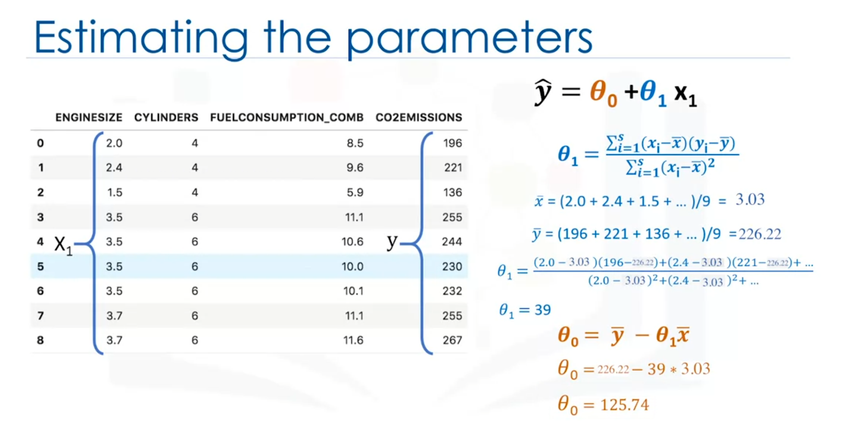
Example Calculation

For a dataset with known values:

• If $θ_1$= 43.98 and $θ_0$ = 92.94, the linear model is:

Prediction Example

For a car with an engine size of 2.4:

Why Linear Regression is Useful

• Simplicity: Easy to use and understand.

• Speed: Fast and efficient.

• No Parameter Tuning: Does not require parameter tuning like other algorithms (e.g., k-nearest neighbors, neural networks).

• Interpretability: Highly interpretable and provides clear insights into relationships between variables.

Model Evaluation in Regression

Model evaluation in regression aims to assess how well a model can predict unknown data. Two main evaluation approaches are commonly used: train and test on the same dataset, and train/test split. Additionally, K-fold cross-validation is introduced as a more advanced method to address some limitations of the other two approaches.

Evaluation Approaches

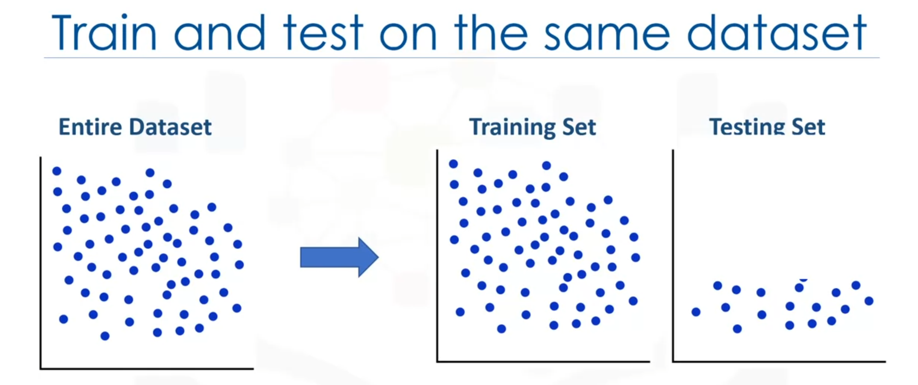
1. Train and Test on the Same Dataset:
   • Process:
     • Use the entire dataset to train the model.
     • Select a portion of the dataset as the test set (without labels during prediction).
     • Predict target values using the model.
     • Compare predicted values with actual values to calculate accuracy.
   • Metrics:
     • Compare actual values y with predicted values $\hat{y}$.
     • Calculate the error as the average difference between predicted and actual values.
   • Advantages:
     • Simple and straightforward.
   • Disadvantages:
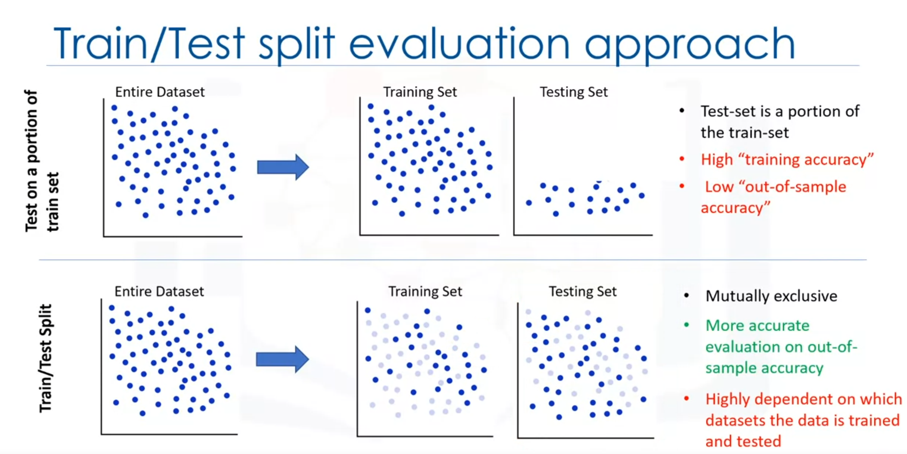
     • High training accuracy but low out-of-sample accuracy due to overfitting.

     

     Code Example:

     from sklearn.linear_model import LinearRegression
     from sklearn.metrics import mean_squared_error
     
     # Example data
     X = [[1, 2], [2, 3], [4, 5], [3, 6]]  # Independent variables
     y = [2, 3, 5, 7]                      # Dependent variable
     
     # Initialize and train the model
     model = LinearRegression()
     model.fit(X, y)
     
     # Predict on the same dataset
     predictions = model.predict(X)
     
     # Calculate training accuracy (MSE)
     mse = mean_squared_error(y, predictions)
     print(f'Mean Squared Error: {mse}')

2. Train/Test Split:
   • Process:
     • Split the dataset into training and testing sets (mutually exclusive).
     • Train the model on the training set.
     • Test the model on the test set by predicting target values.
     • Compare predicted values with actual values to calculate accuracy.
   • Advantages:
     • Provides a better evaluation of out-of-sample accuracy.
     • More realistic for real-world problems.
   • Disadvantages:
     • Dependent on the specific split of the dataset, which can introduce variation.

   

   Code Example:

   from sklearn.model_selection import train_test_split
   
   # Example data
   X = [[1, 2], [2, 3], [4, 5], [3, 6]]  # Independent variables
   y = [2, 3, 5, 7]                      # Dependent variable
   
   # Split the data into training and testing sets
   X_train, X_test, y_train, y_test = train_test_split(X, y, test_size=0.25, random_state=42)
   
   # Train the model
   model = LinearRegression()
   model.fit(X_train, y_train)
   
   # Test the model on the test set
   predictions = model.predict(X_test)
   
   # Calculate out-of-sample accuracy (MSE)
   mse = mean_squared_error(y_test, predictions)
   print(f'Mean Squared Error on Test Set: {mse}')

Key Concepts

• Training Accuracy: The percentage of correct predictions the model makes on the training dataset. High training accuracy may indicate overfitting.

• Out-of-Sample Accuracy: The percentage of correct predictions the model makes on data it has not been trained on. High out-of-sample accuracy indicates better generalization to new data.

K-Fold Cross-Validation

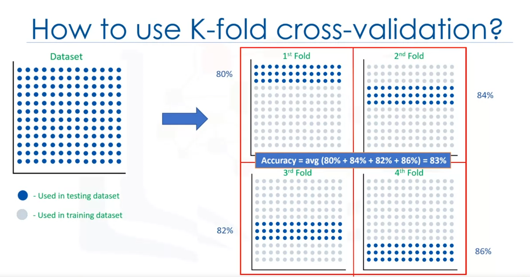
K-fold cross-validation is a method to address the dependency and variation issues in the train/test split approach. It provides a more consistent measure of out-of-sample accuracy by performing multiple train/test splits.

• Process:
  • Divide the dataset into equal folds.
  • For each fold:
    • Use one fold as the test set and the remaining $K−1$ folds as the training set.
    • Train the model on the training set and evaluate it on the test set.
  • Repeat the process for each fold.
  • Average the accuracy results from all folds to obtain a final evaluation metric.

Example with $K=4$

• Split the dataset into 4 equal parts.

• In each iteration, use a different part as the test set and the rest as the training set.

• Compute accuracy for each fold and average the results.

Advantages of K-Fold Cross-Validation:

• Reduces the dependency on a specific train/test split.

• Provides a more reliable estimate of out-of-sample accuracy.

Code Example:

from sklearn.model_selection import cross_val_score

# Example data
X = [[1, 2], [2, 3], [4, 5], [3, 6]]  # Independent variables
y = [2, 3, 5, 7]                      # Dependent variable

# Perform K-Fold Cross-Validation
scores = cross_val_score(model, X, y, cv=4, scoring='neg_mean_squared_error')
mse_scores = -scores
print(f'Mean Squared Error for each fold: {mse_scores}')
print(f'Average Mean Squared Error: {mse_scores.mean()}')

Formula for Mean Squared Error (MSE):

Where $y_i$ are the actual values, $\hat{y}_i$ are the predicted values, and $n$ is the number of observations.

Summary

• Train and Test on the Same Dataset: Simple but prone to overfitting with high training accuracy and low out-of-sample accuracy.

• Train/Test Split: Provides better out-of-sample accuracy but can still be affected by dataset dependency.

• K-Fold Cross-Validation: Mitigates issues of train/test split by averaging results over multiple splits, offering a more consistent evaluation metric.

Model Evaluation Metrics for Regression

Introduction

Evaluation metrics are essential for assessing the performance of a regression model. These metrics compare actual values to predicted values, providing insights into areas needing improvement. Several key metrics are used to evaluate regression models, including Mean Absolute Error (MAE), Mean Squared Error (MSE), Root Mean Squared Error (RMSE), Relative Absolute Error (RAE), Relative Squared Error (RSE), and R-squared ($R^2$).

Error Definition

In regression, the error is the difference between the actual data points and the predicted values from the model. This difference can be measured in various ways.

Mean Absolute Error (MAE)

Mean Absolute Error is the average of the absolute differences between actual and predicted values. It is easy to understand and represents the average error in the same units as the data.

Code Example

from sklearn.metrics import mean_absolute_error

# Example data
y_true = [3, -0.5, 2, 7]
y_pred = [2.5, 0.0, 2, 8]

# Calculate MAE
mae = mean_absolute_error(y_true, y_pred)
print(f"Mean Absolute Error: {mae}")

Mean Squared Error (MSE)

Mean Squared Error is the average of the squared differences between actual and predicted values. It emphasizes larger errors more than smaller ones due to the squaring term, making it more sensitive to outliers.

Code Example

from sklearn.metrics import mean_squared_error

# Calculate MSE
mse = mean_squared_error(y_true, y_pred)
print(f"Mean Squared Error: {mse}")

Root Mean Squared Error (RMSE)

Root Mean Squared Error is the square root of the mean squared error. It is popular because it is in the same units as the response variable, making it easier to interpret.

Code Example

import numpy as np

# Calculate RMSE
rmse = np.sqrt(mse)
print(f"Root Mean Squared Error: {rmse}")

Relative Absolute Error (RAE)

Relative Absolute Error (RAE) is a metric expressed as a ratio normalizing the absolute error. It measures the average absolute difference between the actual and predicted values relative to the average absolute difference between the actual values and their mean.

where $\bar{y}$ is the mean of the actual values.

Code Example

# Calculate RAE
rae = np.sum(np.abs(y_true - y_pred)) / np.sum(np.abs(y_true - np.mean(y_true)))
print(f"Relative Absolute Error: {rae}")

Relative Squared Error (RSE)

Relative Squared Error is similar to RAE but uses squared differences. It is widely adopted for calculating $R^2$.

where $\bar{y}$ is the mean of the actual values.

Code Example

# Calculate RSE
rse = np.sum((y_true - y_pred) ** 2) / np.sum((y_true - np.mean(y_true)) ** 2)
print(f"Relative Squared Error: {rse}")

R-squared ($R^2$)

R-squared is not an error metric per se (by itself), but it is a popular measure of model accuracy. It indicates how close the data points are to the fitted regression line. A higher $R^2$ value indicates a better fit.

where $\bar{y}$ is the mean of the actual values.

Code Example

from sklearn.metrics import r2_score

# Calculate R-squared
r2 = r2_score(y_true, y_pred)
print(f"R-squared: {r2}")

Residual Sum of Squares (RSS)

The Residual Sum of Squares (RSS) is a measure of the discrepancy between the data and an estimation model. It is calculated as the sum of the squared differences between the observed actual outcomes and the outcomes predicted by the model.

Code Example

# Calculate RSS
rss = np.sum((y_true - y_pred) ** 2)
print(f"Residual Sum of Squares: {rss}")

Summary

Each of these metrics quantifies different aspects of model performance. The choice of metric depends on the specific model, data type, and domain knowledge. Understanding and selecting the appropriate metric is crucial for evaluating and improving regression models.

Multiple Linear Regression

Linear Regression Models

• Simple Linear Regression: Utilizes one independent variable to estimate a dependent variable (e.g., predicting CO₂ emissions based on engine size).

• Multiple Linear Regression: Involves multiple independent variables to predict a dependent variable (e.g., predicting CO₂ emissions using engine size and the number of cylinders).

Applications of Multiple Linear Regression

1. Identifying Effect Strength: Determines how independent variables affect the dependent variable. For instance, assessing how revision time, test anxiety, lecture attendance, and gender influence student exam performance.

2. Predicting Impact of Changes: Evaluates how changes in independent variables affect the dependent variable. For example, predicting how a patient's blood pressure changes with variations in body mass index, keeping other factors constant.

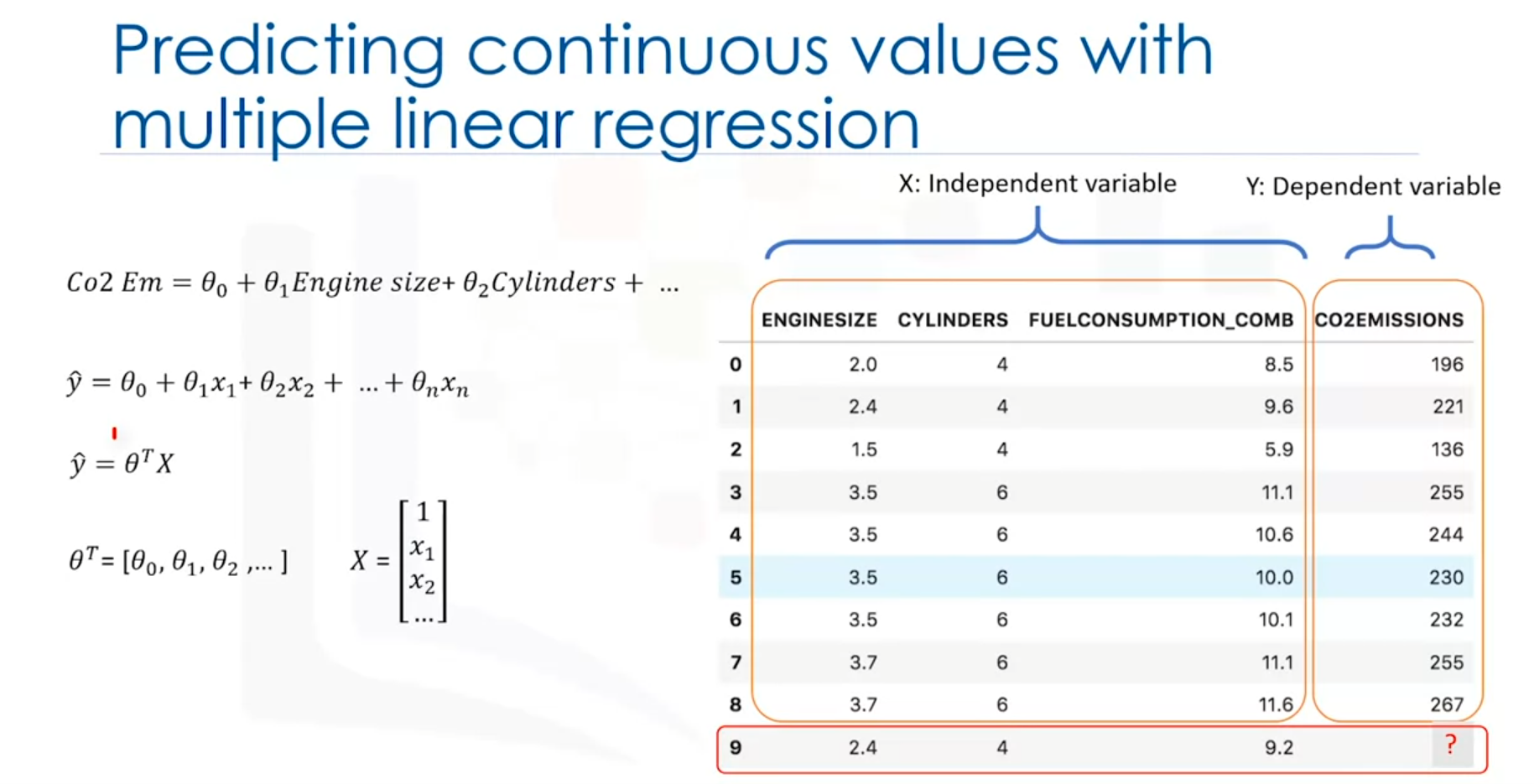
Model Representation

• Equation: The model can be expressed as $\hat{y}=θ_0+θ_1x_1+θ_2x_2+…+θ_nx_n$.

• Vector Form: In multidimensional space, the model is represented as $\theta^T x$, where $θ$ is the vector of parameters and $x$ is the feature set. The first element of $x$ is set to one to account for the intercept ($\theta_0$).

Code Example:

Here’s an example of implementing Multiple Linear Regression in Python using scikit-learn:

from sklearn.linear_model import LinearRegression
import numpy as np

# Example data
X = np.array([[1, 2], [2, 3], [4, 5], [3, 6]])  # Independent variables
y = np.array([2, 3, 5, 7])                      # Dependent variable

# Initialize and fit the model
model = LinearRegression()
model.fit(X, y)

# Coefficients and intercept
print(f'Intercept: {model.intercept_}')
print(f'Coefficients: {model.coef_}')

# Making predictions
predictions = model.predict(X)
print(f'Predictions: {predictions}')

Error and Optimization

• Error Calculation: The error for a prediction is the difference between the actual and predicted values. For example, if the actual value $y$ is 196 and the predicted value $\hat{y}$ is 140, the error is $196−140=56$.

• Mean Squared Error (MSE): The average of the squared errors across all predictions. The objective is to minimize MSE to find the best parameters.

Parameter Estimation Methods

1. Ordinary Least Squares (OLS): Estimates coefficients by minimizing MSE using matrix operations. Suitable for smaller datasets but can be slow for larger ones.

2. Optimization Algorithms: Methods like Gradient Descent iteratively adjust coefficients to minimize error. Suitable for large datasets. Some Optimization Algorithms: Gradient Descent, Stochastic Gradient Descent, Newton’s Metho

Code Example:

Here's a simple implementation of Gradient Descent for linear regression:

import numpy as np

def gradient_descent(X, y, learning_rate=0.01, iterations=1000):
    m, n = X.shape
    theta = np.zeros(n)
    for _ in range(iterations):
        gradient = X.T @ (X @ theta - y) / m
        theta -= learning_rate * gradient
    return theta

# Example data
X = np.array([[1, 2], [2, 3], [4, 5], [3, 6]])  # Independent variables
y = np.array([2, 3, 5, 7])                      # Dependent variable

# Adding intercept term (column of ones)
X_b = np.c_[np.ones((X.shape[0], 1)), X]

# Apply gradient descent
theta = gradient_descent(X_b, y)
print(f'Optimized coefficients: {theta}')

Prediction Phase

• Using Parameters: Once parameters are found, predictions are made by plugging input values into the model equation. For instance, with $\theta_0 = 125$, $\theta_1 = 6.2$, $\theta_2 = 14$, and input values, CO₂ emissions for a car can be predicted.

Concerns in Multiple Linear Regression

• Number of Variables: Adding too many variables without justification can lead to overfitting, where the model becomes too complex and less generalizable.

• Variable Types: Categorical variables can be included by converting them to numerical values (e.g., coding car type as 0 or 1).

• Linearity: Ensure a linear relationship between the dependent variable and independent variables (maybe scatterplot). Non-linear relationships may require non-linear regression.