
Module 3: Classification
Introduction to Classification
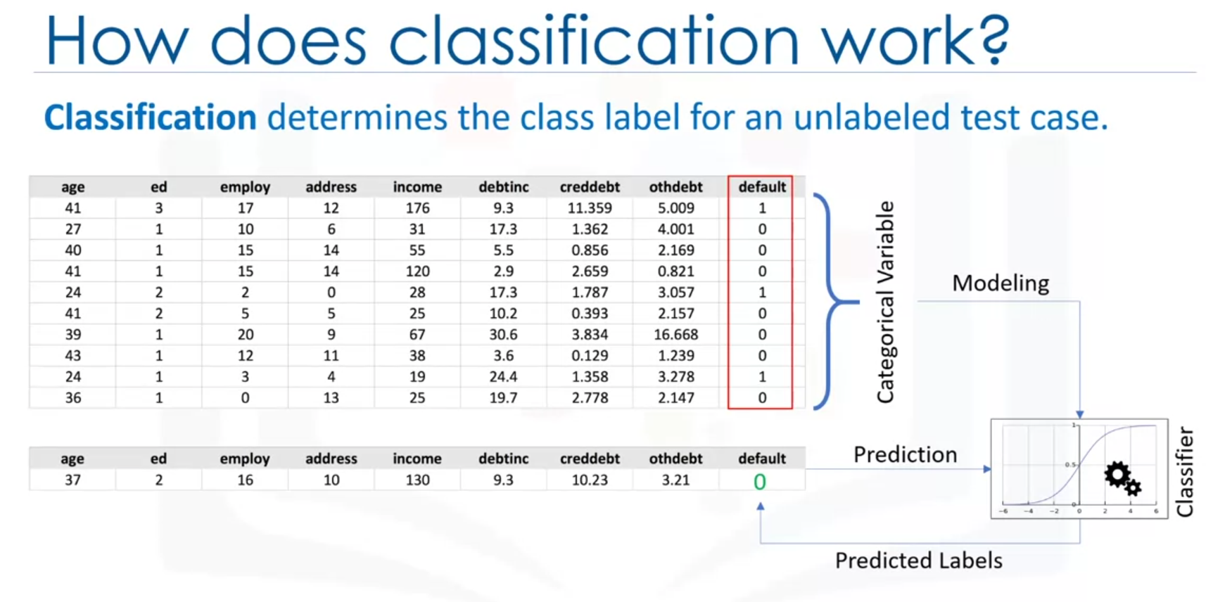
Classification is a supervised learning approach used to categorize items into discrete classes. It aims to learn the relationship between feature variables and a target variable, which is categorical.
How Classification Works
Given training data with target labels, a classification model predicts the class label for new, unlabeled data.
Example:
A loan default predictor uses historical data (e.g., age, income) to classify customers as defaulters or non-defaulters.
Types of Classification
Binary Classification
Predicts one of two possible classes (e.g., defaulter vs. non-defaulter).
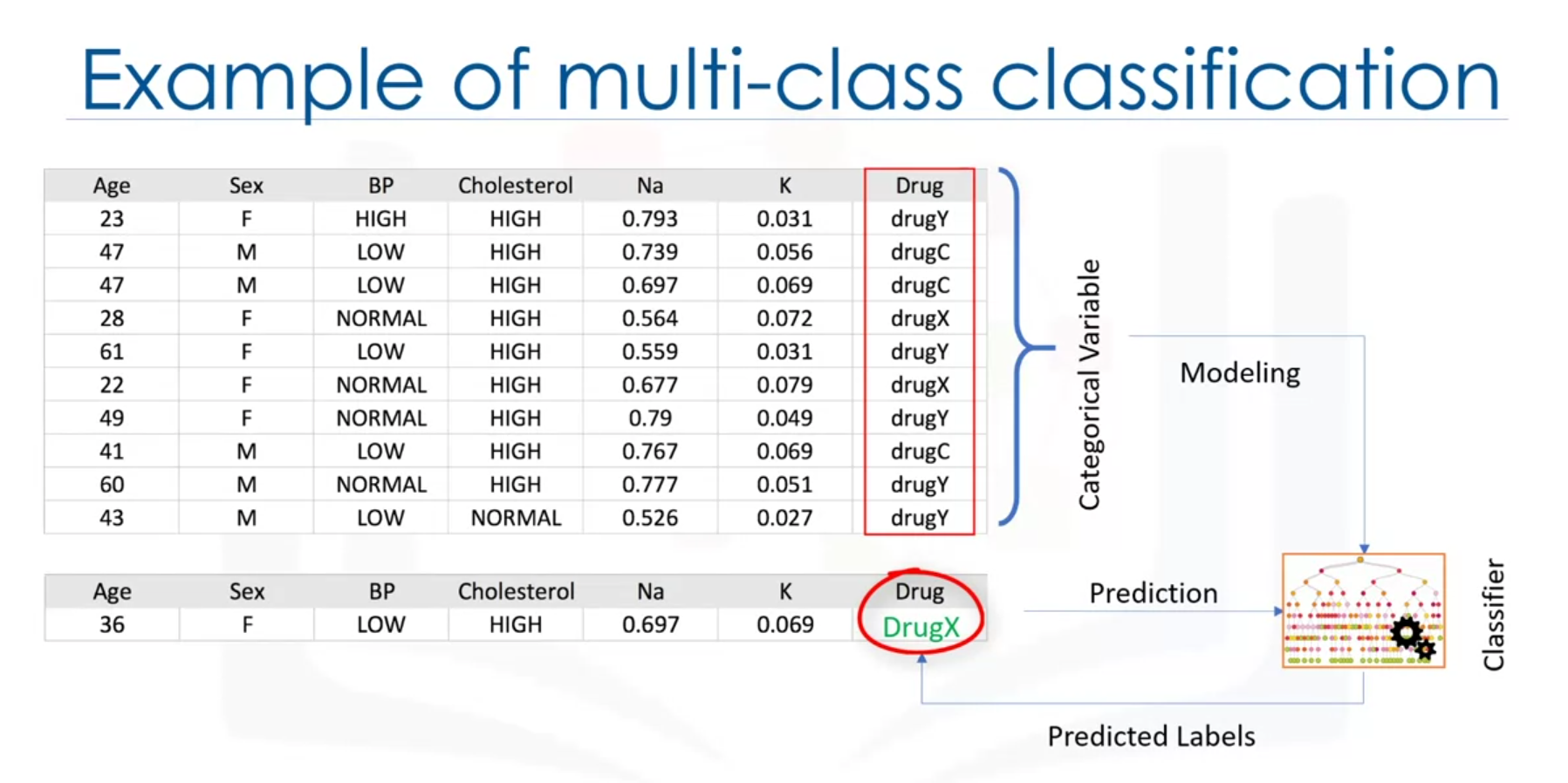
Multi-class Classification
Predicts among more than two classes (e.g., which medication is appropriate for a patient).
Applications
Business Use Cases
- Churn detection
- Customer segmentation
- Response prediction
Industries
- Email filtering
- Speech and handwriting recognition
- Biometric identification
Common Classification Algorithms
- K-Nearest Neighbors (KNN)
- Decision Trees
- Logistic Regression
- Support Vector Machines (SVM)
- Neural Networks
- Naive Bayes
- SoftMax Regression
- One-vs-All (One-vs-Rest)
- One-vs-One
K-Nearest Neighbors (KNN) Algorithm
Overview
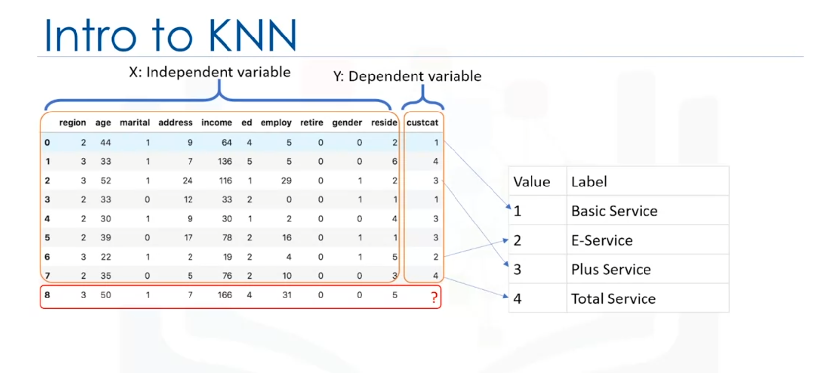
The K-Nearest Neighbors (KNN) algorithm is a supervised learning classification technique used to classify a data point based on how its neighbors are classified. It is based on the concept that data points that are close to each other are more likely to belong to the same class. KNN can also be used for regression tasks.
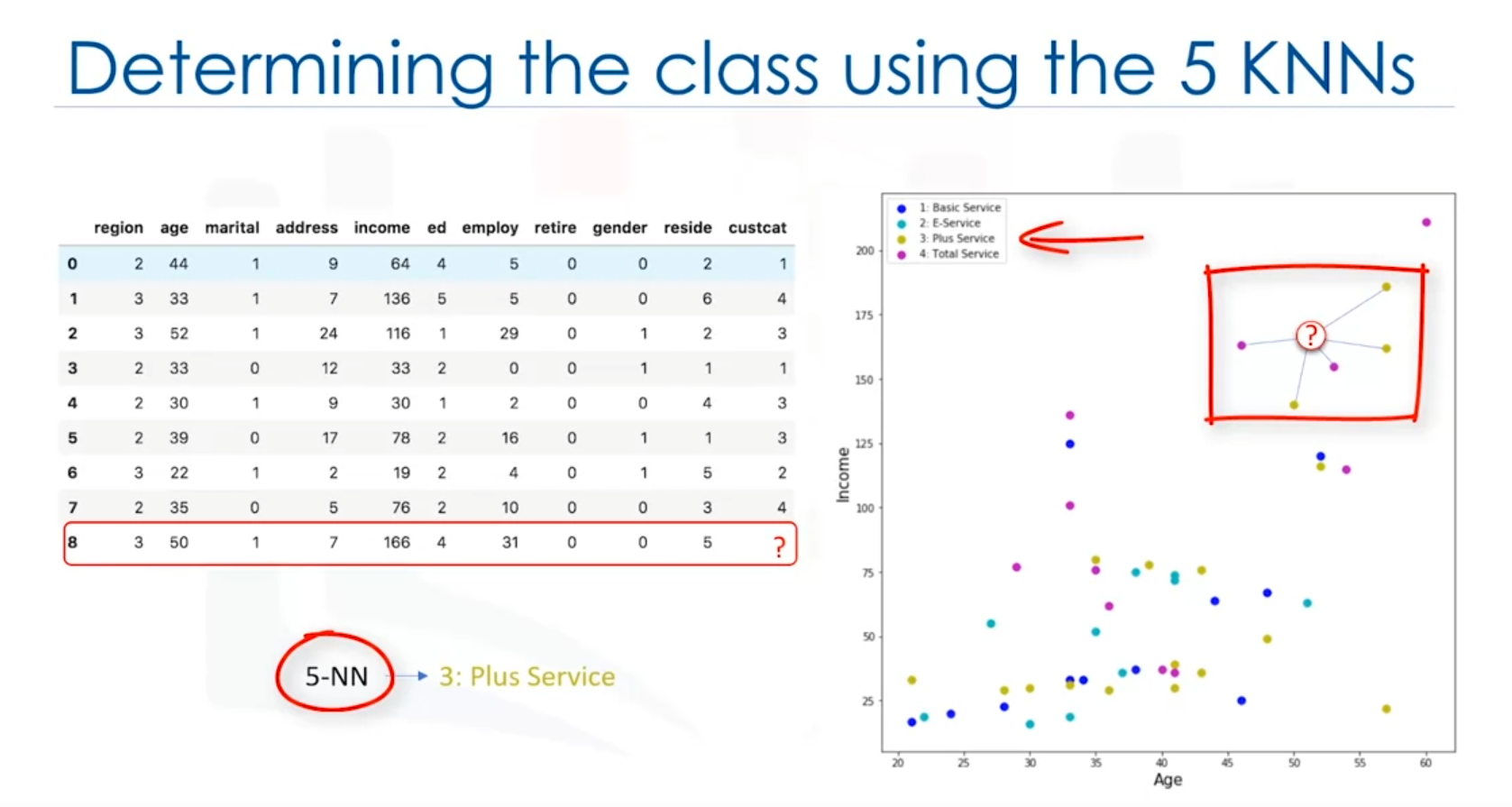
Example Scenario
Consider a telecommunications provider that has segmented its customer base into four groups based on service usage patterns. The goal is to predict which group a new customer belongs to using demographic data such as age and income. This is a classification problem, where the goal is to assign a class label to a new, unknown case based on the known labels of other cases.
How K-Nearest Neighbors Works
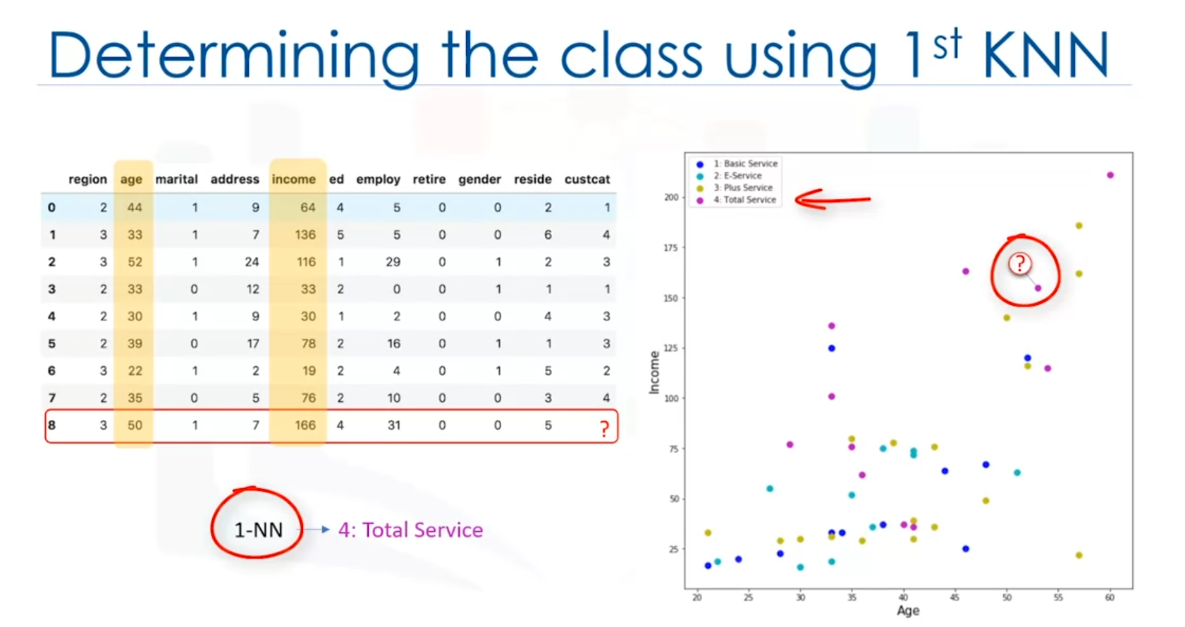
- Choosing the Number of Neighbors (K): The number of neighbors (K) to consider is specified by the user.
- Calculating Distance: For a new data point, the algorithm calculates the distance between this point and all other points in the dataset. Common distance metrics include Euclidean distance.
- Finding the Nearest Neighbors: The K data points that are closest to the new data point are identified.
- Assigning a Class Label: The new data point is assigned the class label that is most common among its K nearest neighbors.
Example of KNN Classification
- Scenario: A new customer’s demographic data (e.g., age and income) is available. The goal is to classify this customer into one of four service groups.
- Process:
- If K=1, the new customer is assigned the same class as the closest existing customer.
- If K=5, the new customer is assigned the class that is most frequent among the 5 nearest neighbors.
Example Code for KNN:
from sklearn.neighbors import KNeighborsClassifier

# Training data
X_train = df[['Age', 'Income']]
y_train = df['Customer Group']

# New customer data
new_customer = [[30, 55000]]

# Initialize KNN classifier
knn = KNeighborsClassifier(n_neighbors=3)

# Fit the model
knn.fit(X_train, y_train)

# Predict the class of the new customer
predicted_class = knn.predict(new_customer)
print(f'Predicted Customer Group: {predicted_class[0]}')
Choosing the Value of K
- Small K: A small value of K (e.g., K=1) might lead to a model that is too specific, potentially capturing noise and outliers. This can result in overfitting, where the model performs well on the training data but poorly on unseen data.
- Large K: A large value of K (e.g., K=20) might make the model too generalized, leading to underfitting, where the model is too simple and fails to capture important patterns in the data.
Finding the Optimal K
To find the optimal value of K:
- Reserve a portion of your data for testing.
- Train the model using the training data and evaluate its accuracy on the test data for different values of K.
- Choose the value of K that results in the highest accuracy.
Example of Choosing K:
from sklearn.model_selection import train_test_split
from sklearn.metrics import accuracy_score

# Split data into training and testing sets
X_train, X_test, y_train, y_test = train_test_split(X_train, y_train, test_size=0.2)

# Evaluate different values of K
accuracies = []
for k in range(1, 11):
    knn = KNeighborsClassifier(n_neighbors=k)
    knn.fit(X_train, y_train)
    y_pred = knn.predict(X_test)
    accuracies.append(accuracy_score(y_test, y_pred))

best_k = accuracies.index(max(accuracies)) + 1
print(f'Best K: {best_k}')
Regression with KNN
KNN can also be used for regression tasks. In this case, instead of assigning a class label, the algorithm predicts a continuous value (e.g., the price of a house). The predicted value is typically the average or median of the K nearest neighbors' values.
Example of KNN Regression
- Scenario: Predicting the price of a house based on features such as the number of rooms, square footage, and the year it was built.
- Process: The algorithm finds the K nearest houses (based on the features) and predicts the price of the new house as the average or median of the prices of these K neighbors.
Summary
The KNN algorithm is a simple yet powerful tool for both classification and regression tasks. Its effectiveness depends on the choice of K and the distance metric used. The main challenge lies in finding the right balance between underfitting and overfitting by selecting an appropriate value of K.
Evaluation Metrics for Classifiers
Model evaluation metrics are essential in determining the performance of a classifier. These metrics provide insights into areas where the model might require improvement. In this note, we will explore three evaluation metrics for classification: Jaccard index, F1 score, and Log Loss.
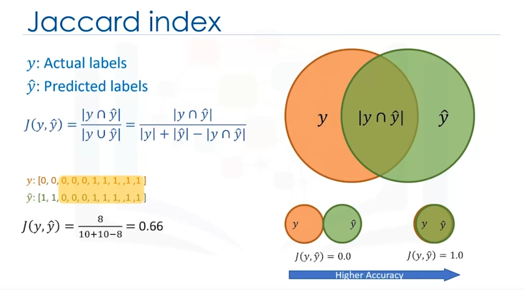
1. Jaccard Index
Definition
The Jaccard index (also known as the Jaccard similarity coefficient) measures the similarity between the actual labels and the predicted labels by the model. It is calculated as the size of the intersection divided by the size of the union of the two label sets.
Formula
Given that y represents the true labels and ŷ represents the predicted labels:
Example
For a test set of size 10 with 8 correct predictions (8 intersections):
Interpretation
- A Jaccard index of 1.0 indicates a perfect match between predicted and true labels.
- A value closer to 0 indicates a poor match.
Code Example
from sklearn.metrics import jaccard_score

# True labels
y_true = [1, 0, 1, 1, 0, 0, 1, 0, 1, 1]

# Predicted labels
y_pred = [1, 0, 1, 0, 0, 1, 1, 0, 1, 0]

# Compute Jaccard Index
jaccard = jaccard_score(y_true, y_pred)
print("Jaccard Index:", jaccard)
2. Confusion Matrix
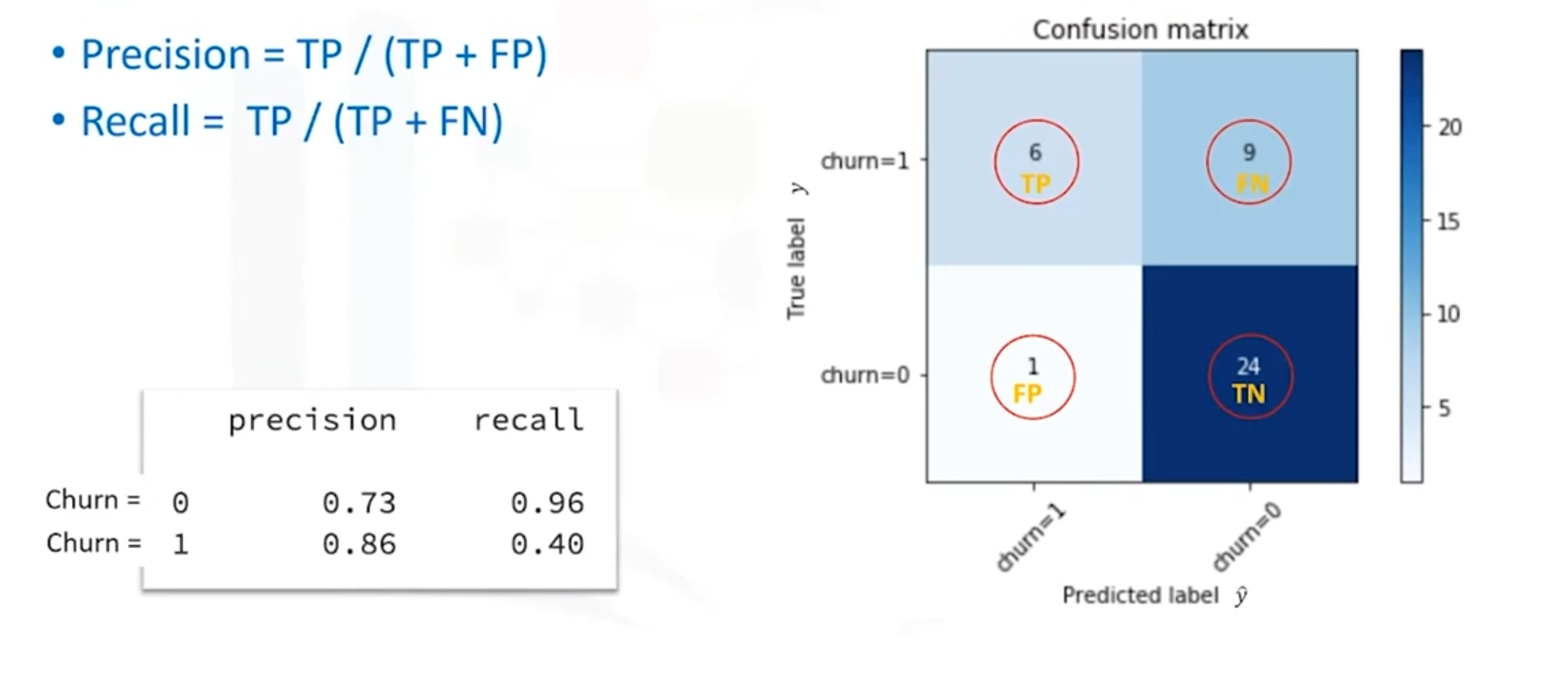
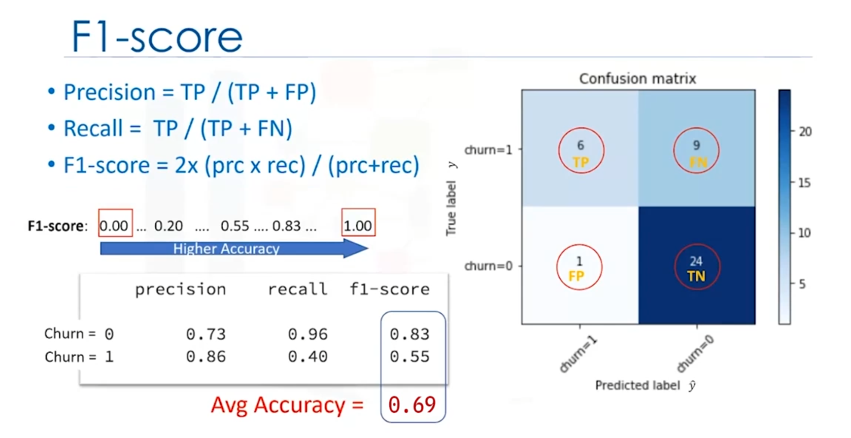
Definition
A confusion matrix is a table that is often used to describe the performance of a classification model on a set of test data for which the true values are known. Each row of the matrix represents the actual instances in a predicted class, while each column represents the instances in an actual class.
Example
Consider a confusion matrix for a binary classification with 40 rows:
| Predicted: No (0) | Predicted: Yes (1) | |
| Actual: No (0) | 24 | 1 |
| Actual: Yes (1) | 9 | 6 |
Interpretation
- True Positives (TP): Correctly predicted positive cases (e.g., Actual Yes = 1, Predicted Yes = 1).
- True Negatives (TN): Correctly predicted negative cases (e.g., Actual No = 0, Predicted No = 0).
- False Positives (FP): Incorrectly predicted positive cases (e.g., Actual No = 0, Predicted Yes = 1).
- False Negatives (FN): Incorrectly predicted negative cases(e.g., Actual Yes=1, Predicted No = 0).
Examples
- True Positives (TP): These are cases where the actual condition is positive (the event has occurred), and the model has correctly predicted it as positive.
- Example: A patient has a disease, and the model correctly predicts that the patient has the disease.
- True Negatives (TN): These are cases where the actual condition is negative (the event has not occurred), and the model has correctly predicted it as negative.
- Example: A transaction is legitimate, and the model correctly predicts that it is not fraudulent.
- False Positives (FP): These are cases where the actual condition is negative (the event has not occurred), but the model incorrectly predicts it as positive.
- Example: A legitimate transaction is incorrectly flagged as fraudulent by the model.
- False Negatives (FN): These are cases where the actual condition is positive (the event has occurred), but the model incorrectly predicts it as negative.
- Example: A patient has a disease, but the model incorrectly predicts that the patient does not have the disease.
Precision and Recall
- Precision: The accuracy of the positive predictions. It is calculated as:
- Recall: The true positive rate, measuring the proportion of actual positives correctly identified. It is calculated as:
Code Example
from sklearn.metrics import confusion_matrix

# True labels
y_true = [0, 0, 0, 1, 1, 0, 1, 1, 0, 1]

# Predicted labels
y_pred = [0, 0, 0, 1, 0, 0, 1, 0, 1, 1]

# Compute Confusion Matrix
conf_matrix = confusion_matrix(y_true, y_pred)
print("Confusion Matrix:\n", conf_matrix)
3. F1 Score
Definition
The F1 score is the harmonic mean of precision and recall, providing a balance between the two. It is particularly useful when the class distribution is imbalanced.
Formula
Example
- F1 Score for Class 0 (Churn = No): 0.83
- F1 Score for Class 1 (Churn = Yes): 0.55
- Average F1 Score: 0.69
Interpretation
- An F1 score of 1 indicates perfect precision and recall.
- A lower F1 score indicates poorer performance.
Code Example
from sklearn.metrics import f1_score
# True labels
y_true = [0, 0, 0, 1, 1, 0, 1, 1, 0, 1]
# Predicted labels
y_pred = [0, 0, 0, 1, 0, 0, 1, 0, 1, 1]
# Compute F1 Score
f1 = f1_score(y_true, y_pred)
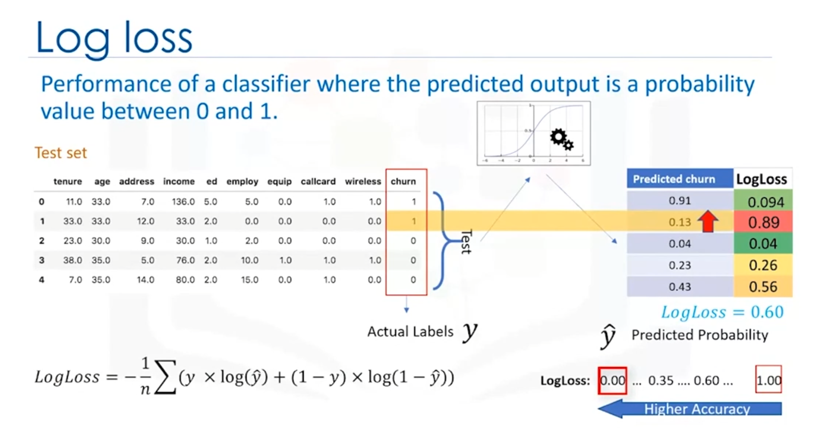
print("F1 Score:", f1)4. Log Loss (Logarithmic Loss)
Definition
Log Loss measures the accuracy of a classifier that outputs probabilities rather than class labels. It penalizes predictions that are confident but wrong more than those that are less confident but wrong.
Formula
Where:
- is the number of observations.
- is the actual label (0 or 1).
- is the predicted probability of the positive class.
Interpretation
- Lower Log Loss: Better accuracy. Indicates that the predicted probabilities are close to the actual labels.
- Higher Log Loss: Worse accuracy. Indicates that the predicted probabilities are far from the actual labels.
Code Example
from sklearn.metrics import log_loss

# True labels
y_true = [0, 0, 0, 1, 1, 0, 1, 1, 0, 1]

# Predicted probabilities
y_prob = [0.1, 0.4, 0.2, 0.8, 0.6, 0.2, 0.9, 0.4, 0.7, 0.8]

# Compute Log Loss
logloss = log_loss(y_true, y_prob)
print("Log Loss:", logloss)
5. Accuracy
Definition
Accuracy measures the proportion of correctly predicted instances (both true positives and true negatives) out of the total number of instances. It is a simple and widely used metric for classification tasks.
Formula
Alternatively, it can also be expressed as:
Example
If a model has 24 true negatives, 6 true positives, 1 false positive, and 9 false negatives, the accuracy is:
Interpretation
- Higher Accuracy: Indicates better overall performance of the model.
- Lower Accuracy: Suggests that the model might be missing some predictions or making incorrect predictions.
Code Example
from sklearn.metrics import accuracy_score

# True labels
y_true = [0, 1, 0, 1, 1, 0, 1, 0, 0, 1]

# Predicted labels
y_pred = [0, 1, 0, 0, 1, 0, 1, 0, 1, 1]

# Compute Accuracy
accuracy = accuracy_score(y_true, y_pred)
print("Accuracy:", accuracy)
Summary
- Jaccard Index: Measures the similarity between actual and predicted labels.
- Confusion Matrix: Provides a detailed breakdown of true positives, true negatives, false positives, and false negatives.
- F1 Score: Balances precision and recall, especially useful for imbalanced datasets.
- Log Loss: Evaluates the accuracy of probabilistic predictions, with lower values indicating better performance.
- Accuracy: Measures the overall proportion of correct predictions, providing a general assessment of the model's performance.
Introduction to Decision Trees
Decision trees are a powerful tool in classification that helps in making decisions based on data. In this note, we will explore what a decision tree is, how it is used for classification, and the basic process of building a decision tree.
1. What is a Decision Tree?
A decision tree is a flowchart-like structure that is used for decision-making. It helps in classifying a dataset by breaking it down into smaller and smaller subsets while at the same time, an associated decision tree is incrementally developed.
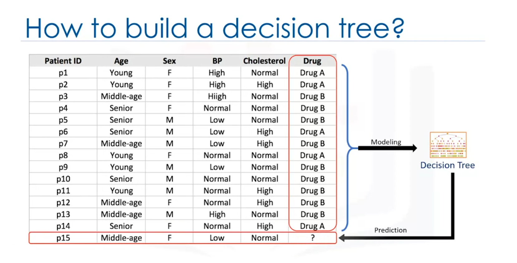
Example Scenario:
Imagine a medical researcher compiling data about patients who suffered from the same illness. The patients responded to one of two medications: Drug A or Drug B. The dataset includes features like age, gender, blood pressure, and cholesterol levels, with the target being the drug each patient responded to.
The goal is to build a model that predicts which drug might be appropriate for a future patient with the same illness. This is a binary classification problem where the decision tree will help classify the appropriate drug.
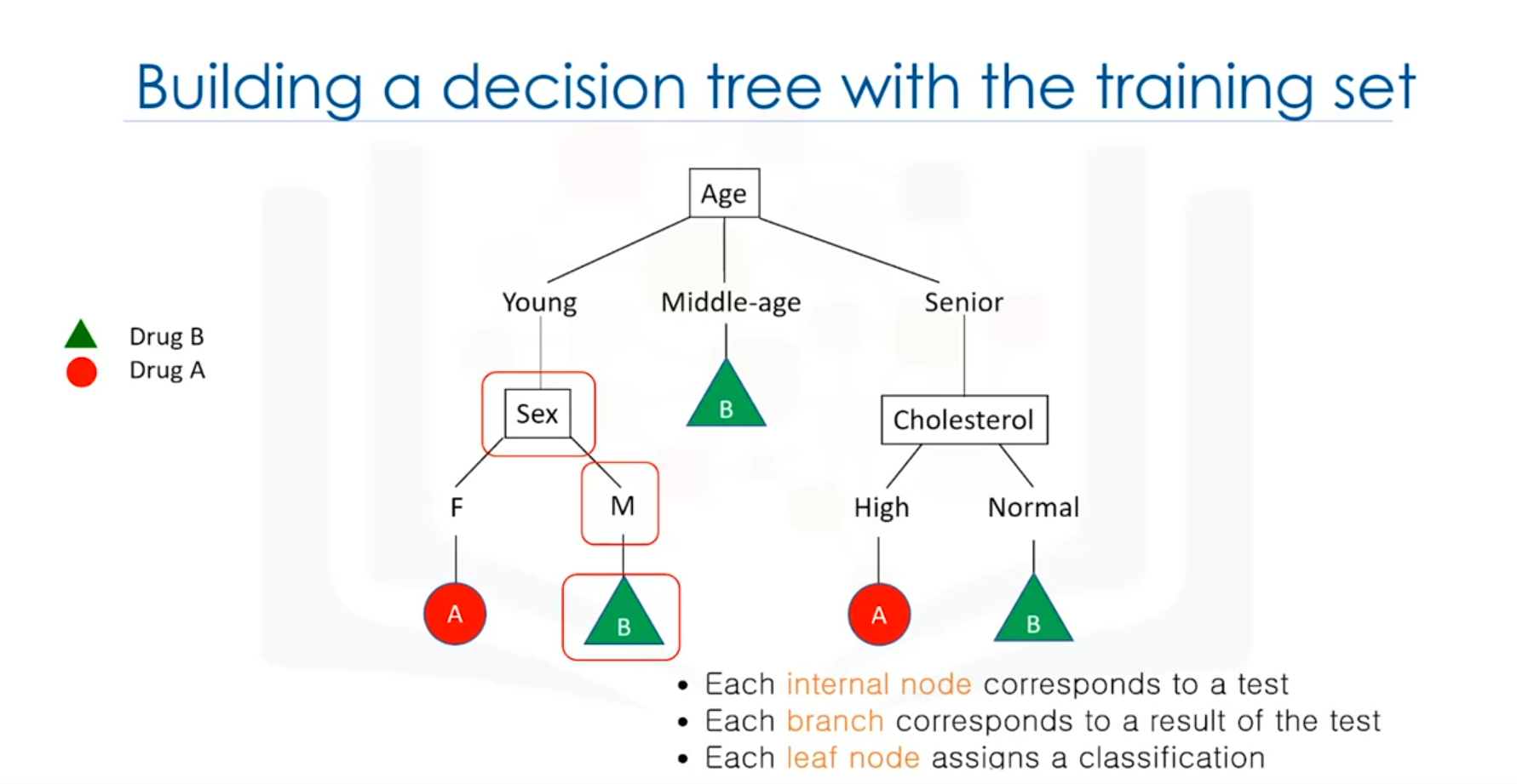
2. Structure of a Decision Tree
Components:
- Root Node: The starting point of the tree, representing the entire dataset.
- Internal Nodes: Represent tests or decisions based on an attribute (e.g., age).
- Branches: Represent the outcomes of a test and lead to the next node or leaf.
- Leaf Nodes: Represent the final decision or classification (e.g., Drug A or Drug B).
Example:
Consider the dataset with features like age, gender, blood pressure, and cholesterol. The decision tree may start with the age attribute:
- Age: If the patient is middle-aged, the tree may directly suggest Drug B.
- Gender: If the patient is young or senior, the next decision might be based on gender, where a female may be prescribed Drug A and a male Drug B.
Each internal node tests an attribute, and the branches represent the possible outcomes of the test. The leaf node assigns the final decision, such as prescribing a specific drug.
3. Building a Decision Tree
Steps Involved:
- Choosing an Attribute: Select an attribute from the dataset (e.g., age).
- Calculating Significance: Determine the significance of the attribute in splitting the data. This significance helps in identifying the best attribute to split the data on.
- Splitting the Data: Based on the value of the chosen attribute, split the data into different branches.
- Repeating the Process: For each branch, repeat the process for the remaining attributes until all attributes are used, or a decision can be made.
Outcome:
Once the tree is built, it can be used to predict the class of new or unknown cases. In the context of our example, the tree can help in determining the appropriate drug for a new patient based on their characteristics.
Key Points:
- Attribute Testing: Decision trees work by testing attributes and making decisions based on the outcomes of these tests.
- Decision-Making: The tree branches based on the results of these tests and assigns a final classification at the leaf nodes.
Summary
- Decision Trees are used for classification by breaking down a dataset into smaller subsets.
- The tree structure includes root nodes, internal nodes, branches, and leaf nodes.
- Building a Decision Tree involves choosing attributes, calculating their significance, and splitting the data until a decision can be made.
Decision trees are intuitive and powerful, especially in scenarios where a clear decision-making process is needed based on multiple attributes.
Decision Tree Building Process
Introduction
Decision trees are a key tool in machine learning used for classification tasks. They work by recursively partitioning data based on the most predictive features, creating branches that lead to decision outcomes.
Recursive Partitioning
The process of building a decision tree involves recursive partitioning, where data is split based on the most predictive features. This splitting continues until the subsets of data (or leaves) are sufficiently pure.
Attribute Selection
Choosing the right attribute for splitting the data is crucial. The effectiveness of an attribute is measured by its ability to reduce impurity in the resulting nodes.
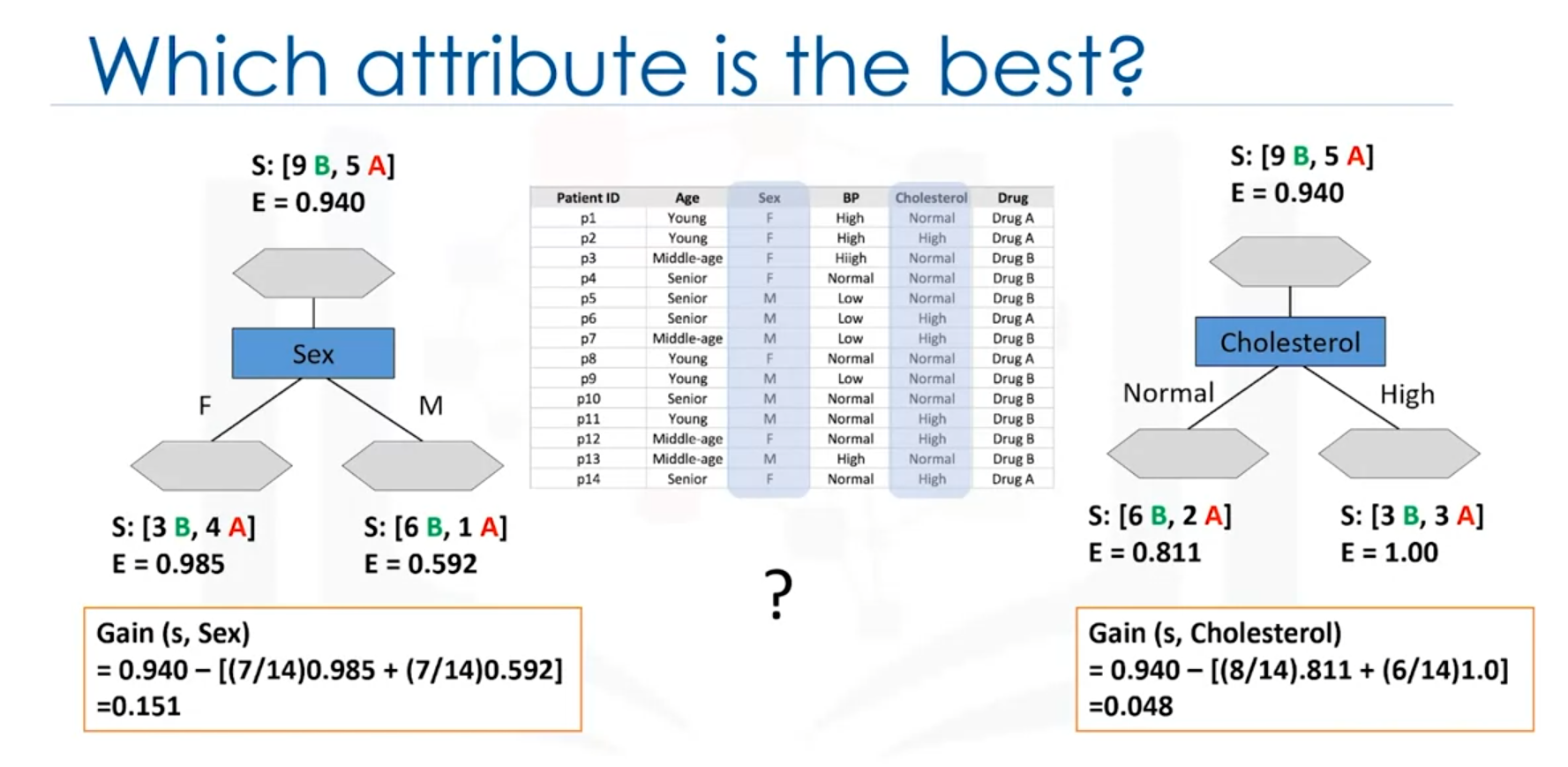
Example: Drug Dataset
Consider a dataset with 14 patients where the goal is to decide which drug to prescribe.
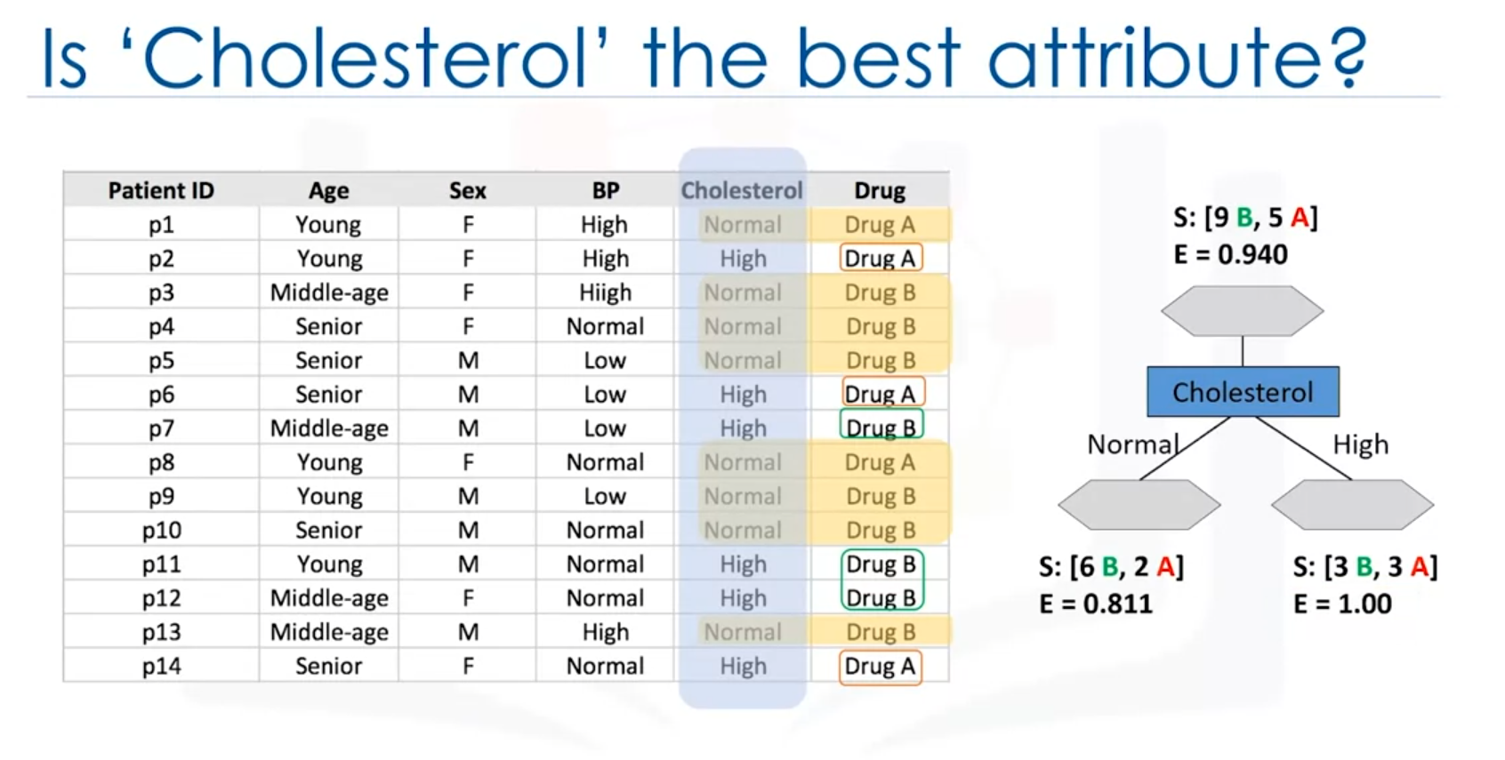
- Cholesterol Attribute: If the split is based on cholesterol levels, the resulting groups might not provide clear decisions:
- High cholesterol: The decision about which drug is suitable is uncertain.
- Normal cholesterol: Similarly, it does not clearly indicate the appropriate drug.
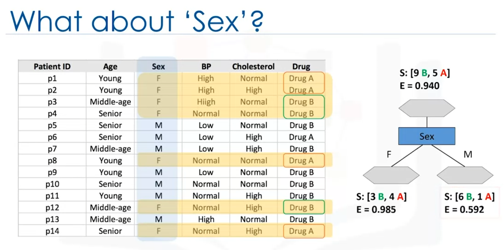
- Sex Attribute: Using the sex attribute to split the data results in:
- Female patients: Drug B might be more suitable.
- Male patients: Further testing with cholesterol levels is needed.
Impurity and Entropy
The purity of a node in a decision tree is assessed using entropy, which measures the randomness or disorder in the data.
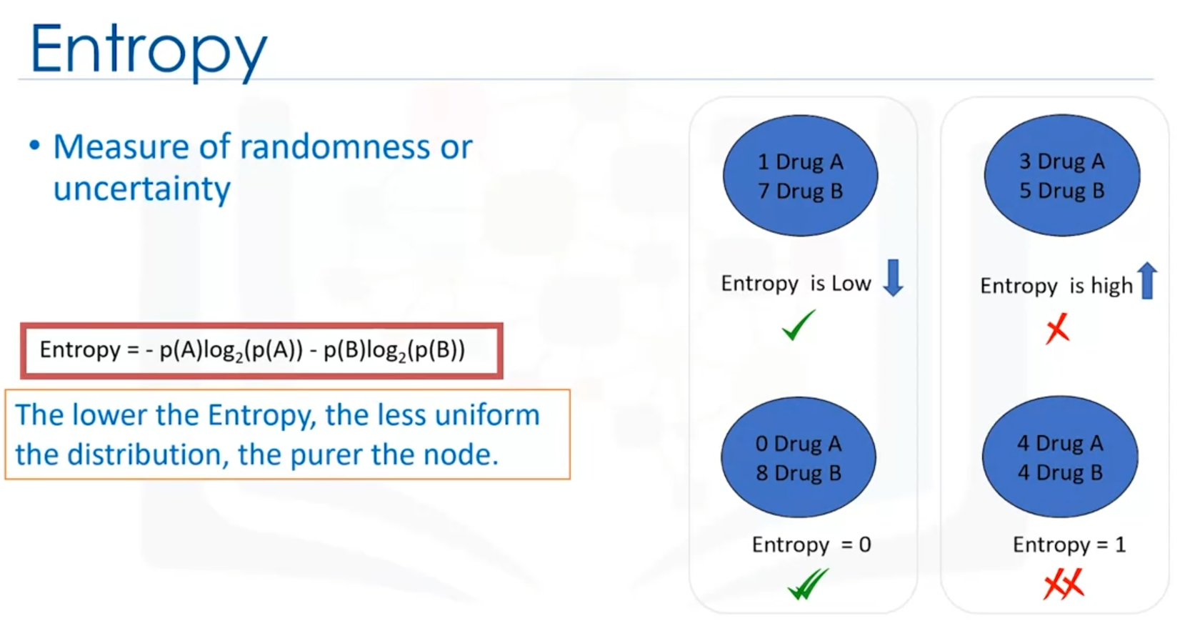
Entropy Calculation
- Definition: Entropy quantifies the level of disorder in a node. A node is considered pure if it contains data from only one class (entropy = 0). If the data is evenly distributed between classes, entropy is 1.
- Formula: Entropy can be calculated using the formula:
where is the proportion of data points belonging to class .
Example Calculation
- Before Splitting: For 9 occurrences of drug B and 5 of drug A, the entropy is 0.94.
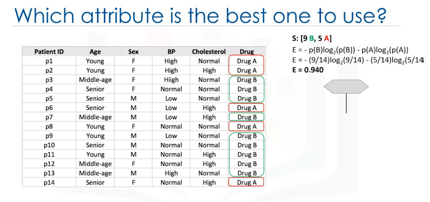
- After Splitting:
- Cholesterol:
- Normal: 6 drug B, 2 drug A (Entropy = 0.8)
- High: 3 drug B, 3 drug A (Entropy = 1.0)
- Sex:
- Female: 3 drug B, 4 drug A (Entropy = 0.98)
- Male: 6 drug B, 1 drug A (Entropy = 0.59)
- Cholesterol:
Information Gain
Information gain measures how well an attribute separates the data into pure subsets. It is calculated as the difference between entropy before and after the split.
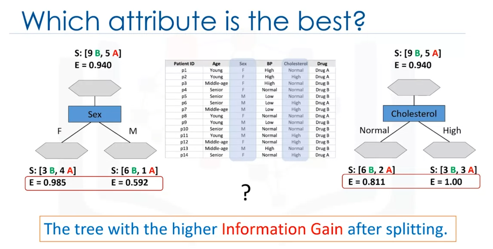
Calculation
- Formula:
- Formula for Weighted Entropy:
where is the proportion of samples in subset , and Entropy is the entropy of subset
- Example:
- Sex Attribute: Information gain = 0.151
- Cholesterol Attribute: Information gain = 0.48x`
Decision Tree Example Using Python
Here's how to create and visualize a decision tree using Python and scikit-learn.
Code Example
import pandas as pd
from sklearn.tree import DecisionTreeClassifier, plot_tree
import matplotlib.pyplot as plt

# Sample dataset
data = {
    'Cholesterol': ['Normal', 'High', 'Normal', 'High', 'Normal', 'High', 'Normal', 'Normal', 'High', 'High', 'Normal', 'High', 'Normal', 'High'],
    'Sex': ['Male', 'Female', 'Female', 'Male', 'Female', 'Male', 'Female', 'Male', 'Male', 'Female', 'Female', 'Male', 'Male', 'Female'],
    'Drug': ['A', 'B', 'A', 'A', 'B', 'B', 'A', 'B', 'B', 'B', 'A', 'A', 'B', 'B']
}
df = pd.DataFrame(data)

# Convert categorical features to numeric
df['Cholesterol'] = df['Cholesterol'].map({'Normal': 0, 'High': 1})
df['Sex'] = df['Sex'].map({'Male': 0, 'Female': 1})
df['Drug'] = df['Drug'].map({'A': 0, 'B': 1})

# Features and target
X = df[['Cholesterol', 'Sex']]
y = df['Drug']

# Initialize and fit the model
clf = DecisionTreeClassifier(criterion='entropy')
clf.fit(X, y)

# y_pred = clf.predit(x_test)

# Plot the decision tree
plt.figure(figsize=(12,8))
plot_tree(clf, feature_names=['Cholesterol', 'Sex'], class_names=['Drug A', 'Drug B'], filled=True)
plt.title('Decision Tree')
plt.show()
Explanation
- Dataset Creation: A sample dataset is created and converted into a DataFrame.
- Feature Encoding: Categorical features are mapped to numeric values.
- Model Training: A
DecisionTreeClassifieris initialized with entropy as the criterion and fitted to the data.
- Visualization: The
plot_treefunction visualizes the trained decision tree.
Conclusion
The attribute with the highest information gain is chosen for splitting the data. In this case, cholesterol has a higher information gain than sex, making it a better choice for the initial split.
This process is repeated for each branch of the tree until the data in each node is sufficiently pure.