Module 4: Linear Classification

Logistic Regression: An Overview

Introduction

Logistic Regression is a statistical and machine learning technique used for classification tasks. This method is particularly useful when predicting a categorical outcome based on one or more independent variables. In this note, we will cover the following key aspects of logistic regression:

What is Logistic Regression?

What kind of problems can be solved by Logistic Regression?

In which situations is Logistic Regression used?

1. What is Logistic Regression?

Logistic Regression is a classification algorithm that models the probability of a binary outcome based on one or more predictor variables. Unlike linear regression, which predicts continuous values, logistic regression is used to predict binary or categorical outcomes, often represented as 0 or 1, yes/no, true/false, etc. Note that logistic regression can be used both for binary classification and multiclass classification.

Example:

Consider a telecommunication dataset where the goal is to predict customer churn. Here, logistic regression can be used to build a model that predicts whether a customer will leave the company based on features such as tenure, age, and income.

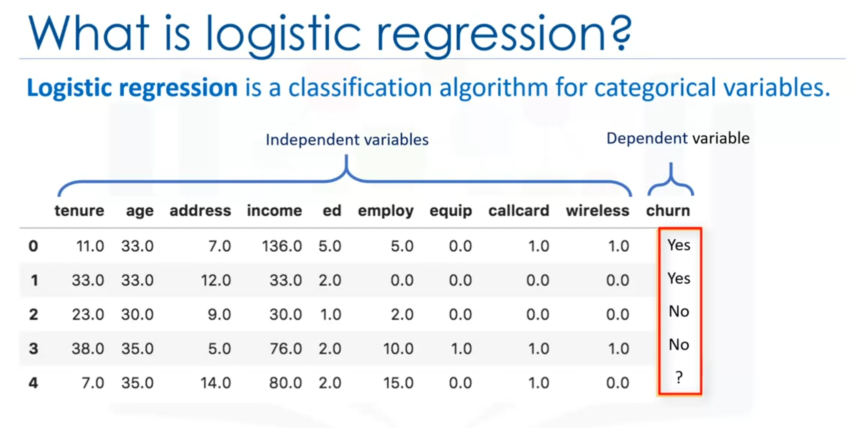
Note: Independent variables should be numerical (continuous value).

2. Problems Solved by Logistic Regression

Logistic regression is widely used for various classification tasks, including:

Medical Diagnosis: Predicting the probability of a patient having a disease based on factors like age, blood pressure, and test results.

Customer Behavior: Estimating the likelihood of a customer making a purchase or canceling a subscription.

Risk Assessment: Predicting the probability of loan default or system failure.

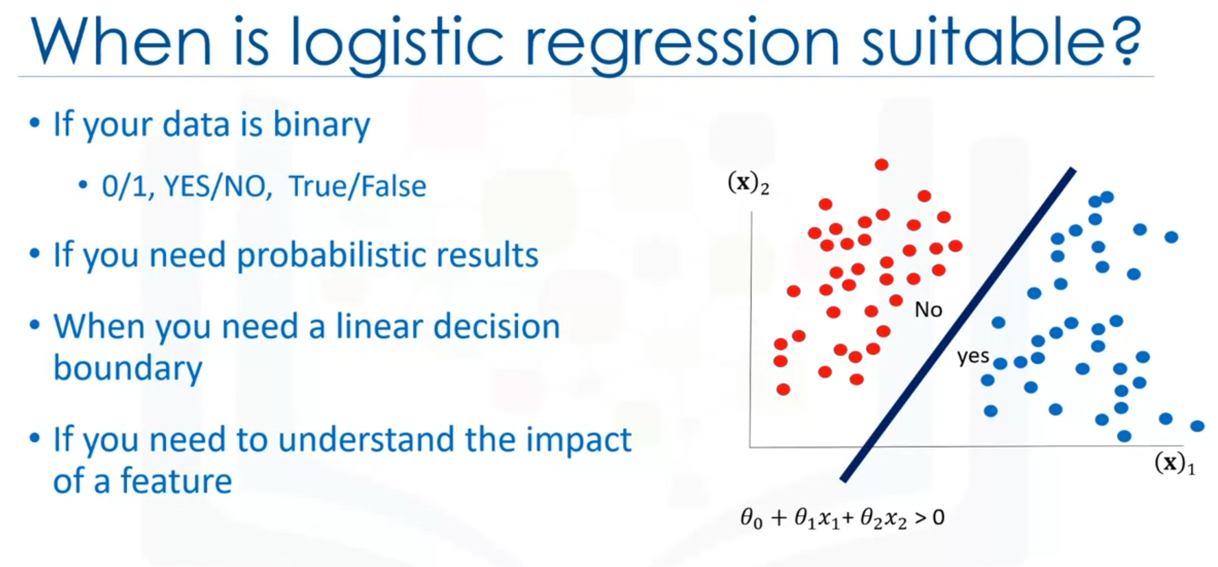
3. Situations to Use Logistic Regression

Logistic regression is an ideal choice in the following scenarios:

Binary Target Field: When the dependent variable is binary (e.g., churn/no churn, positive/negative).

Probability Prediction: When you need the probability of the prediction, such as estimating the likelihood of a customer buying a product.

Linearly Separable Data: When the data is linearly separable, meaning that the decision boundary can be represented as a line or hyperplane.

Feature Impact Analysis: When you need to understand the impact of each feature on the outcome, using the model's coefficients.\

4. How Logistic Regression Works

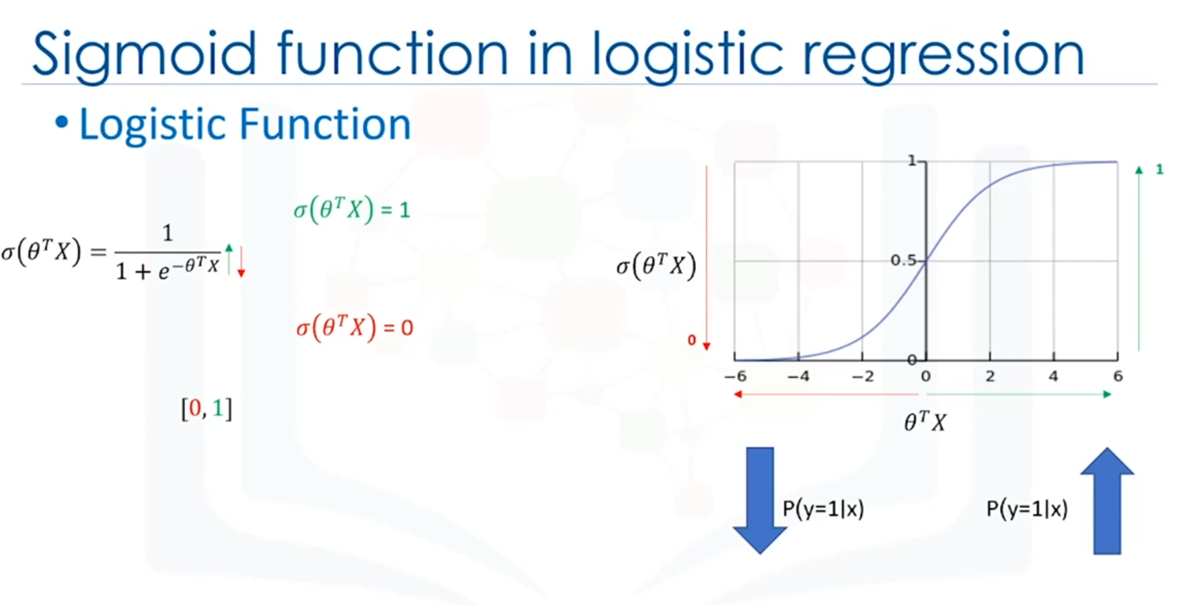
In logistic regression, the relationship between the independent variables (X) and the probability of the dependent variable (Y) is modeled using a logistic function. The logistic function maps any real-valued number into a value between 0 and 1, which can be interpreted as a probability.

Decision Boundary:

Linear Decision Boundary: The model creates a decision boundary that separates the data points into two classes.

Complex Decision Boundary: Logistic regression can also model more complex boundaries by using polynomial features (not covered here).

Example with a Simple Logistic Regression Model:

Dataset (X): Features such as tenure, age, and income.

Target (Y): Whether the customer churns (0 or 1).

Model: The logistic regression model predicts the probability of a customer churning based on the given features.

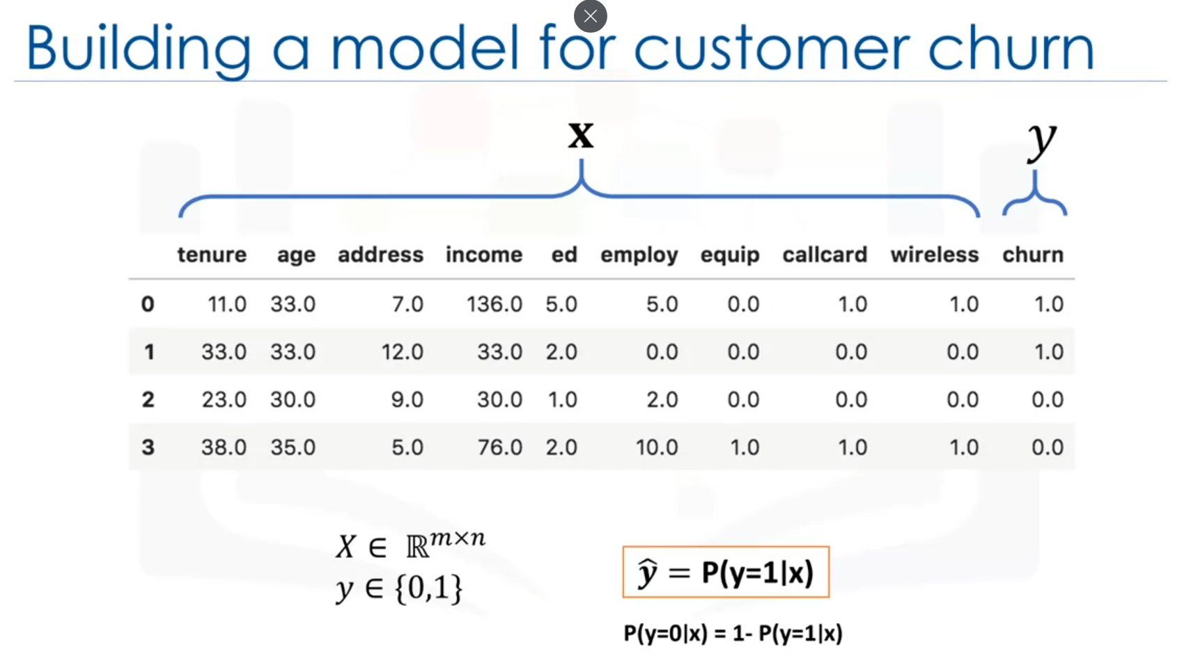
5. Formalizing the Problem

Given a dataset $X$ of $m$ dimensions (features) and $n$ records, and a target variable $Y$ (which can be 0 or 1), the logistic regression model predicts the class of each sample and the probability of it belonging to a particular class.

$X$ : Independent variables (features).

$Y$ : Dependent variable (class label).

$\hat{Y}$ : Predicted class probability.

Conclusion

Logistic regression is a powerful and widely used technique for binary classification problems. It not only predicts the class of each data point but also provides the probability associated with the prediction. This makes it a valuable tool for decision-making in various fields, including healthcare, finance, and marketing.

Introduction to Linear Regression vs. Logistic Regression

Linear Regression Overview

Linear regression is commonly used to predict a continuous variable. For example, suppose the goal is to predict the income of customers based on their age. In this scenario, age is the independent variable (denoted as $x_1$ ), and income is the dependent variable (denoted as $y$ ). The linear regression model fits a line through the data, represented by the equation:

y=a+bx_1

This equation can be used to predict income for any given age.

Python Example: Linear Regression

import numpy as np
import matplotlib.pyplot as plt
from sklearn.linear_model import LinearRegression

# Sample data
ages = np.array([25, 30, 35, 40, 45, 50, 55, 60]).reshape(-1, 1)
incomes = np.array([25000, 30000, 35000, 40000, 45000, 50000, 55000, 60000])

# Create and fit the model
model = LinearRegression()
model.fit(ages, incomes)

# Predicting income for a given age
age_new = np.array([[40]])
predicted_income = model.predict(age_new)
print(f"Predicted income for age 40: ${predicted_income[0]:.2f}")

# Plotting the regression line
plt.scatter(ages, incomes, color='blue')
plt.plot(ages, model.predict(ages), color='red')
plt.xlabel('Age')
plt.ylabel('Income')
plt.title('Linear Regression: Age vs. Income')
plt.show()

Challenges with Linear Regression for Classification

When using linear regression for classification tasks, such as predicting customer churn (a binary outcome: yes or no), the model may predict values outside the [0, 1] range. This can create challenges, as linear regression is not inherently designed to handle classification problems.

For instance, if the goal is to predict whether a customer will churn based on their age, mapping categorical values to integers (e.g., yes = 1, no = 0) and applying linear regression may lead to inaccurate predictions. The model might predict probabilities that are not realistic (e.g., greater than 1 or less than 0).

Introduction to Logistic Regression

Logistic regression is specifically designed for classification problems. It models the probability that an input $x$ belongs to a particular class. Unlike linear regression, logistic regression uses the sigmoid function, which is defined as:

\text{Sigmoid}(\Theta^T x) = \frac{1}{1 + e^{-\Theta^T x}}

Here, $\Theta^T x$ represents the linear combination of features, and the sigmoid function outputs a value between 0 and 1, representing the probability that the input belongs to the positive class (e.g., churn = yes).

Python Example: Logistic Regression

import numpy as np
from sklearn.linear_model import LogisticRegression
from sklearn.model_selection import train_test_split
from sklearn.metrics import accuracy_score

# Sample data: Age and Churn (1 = Yes, 0 = No)
ages = np.array([25, 30, 35, 40, 45, 50, 55, 60]).reshape(-1, 1)
churn = np.array([0, 0, 0, 0, 1, 1, 1, 1])

# Split the data into training and testing sets
X_train, X_test, y_train, y_test = train_test_split(ages, churn, test_size=0.2, random_state=42)

# Create and fit the model
log_reg = LogisticRegression()
log_reg.fit(X_train, y_train)

# Predicting churn for a given age
age_new = np.array([[40]])
predicted_churn = log_reg.predict_proba(age_new)[:, 1]
print(f"Predicted probability of churn for age 40: {predicted_churn[0]:.2f}")

# Model accuracy
y_pred = log_reg.predict(X_test)
print(f"Model accuracy: {accuracy_score(y_test, y_pred):.2f}")

Key Properties of the Sigmoid Function

Range: The output of the sigmoid function is always between 0 and 1, making it suitable for probability estimation.

Interpretation: A higher output value indicates a higher probability that the input belongs to the positive class.

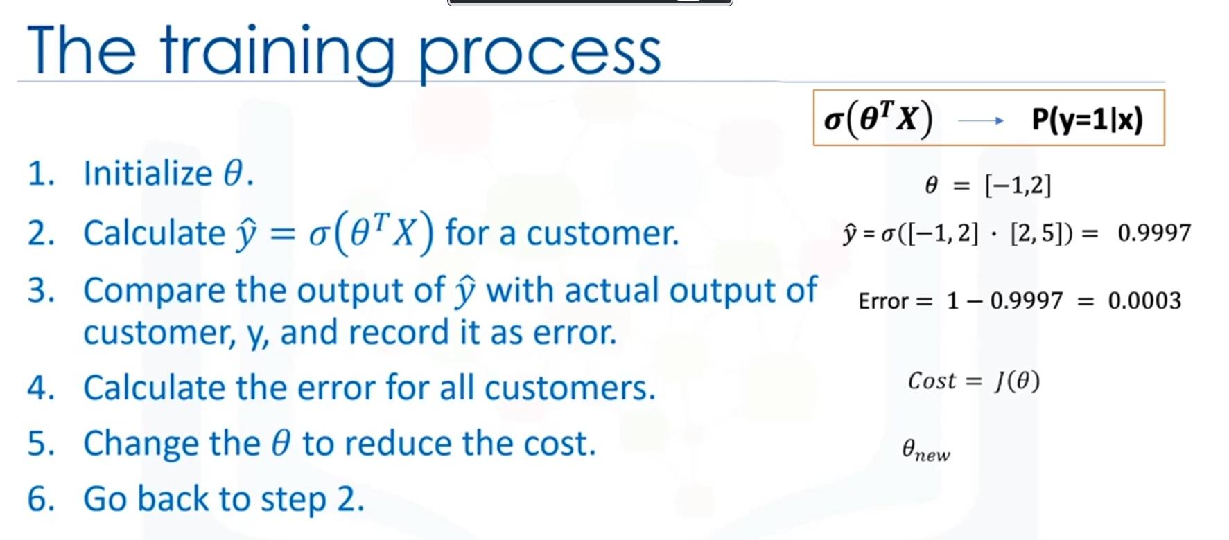
Training the Logistic Regression Model

Training a logistic regression model involves finding the optimal values of the parameter vector $\Theta$ to accurately estimate the probability of each class. The process generally involves the following steps:

Initialization: Start with random values for $\Theta$ .

Model Output: Calculate the sigmoid of $\Theta^T x$ for each sample.

Error Calculation: Compare the predicted probability ( $\hat{y}$ ) with the actual label ( $y$ ) to compute the error.

Cost Function: Aggregate the errors across all samples to calculate the total cost.

Parameter Update: Adjust $\Theta$ to minimize the cost using optimization techniques like gradient descent.

Iteration: Repeat the process until the cost is sufficiently low and the model accuracy is satisfactory.

Conclusion

Logistic regression is a powerful tool for binary and multi-class classification problems. By applying the sigmoid function to a linear model, logistic regression transforms it into a probabilistic model, making it highly effective for tasks that require predicting the likelihood of an outcome.

Training a Logistic Regression Model

Objective of Training in Logistic Regression

The main objective of training a logistic regression model is to adjust the model parameters (weights) to best estimate the labels of the samples in the dataset. This involves understanding and minimizing the cost function to improve the model's performance.

Example: Customer Churn Prediction

In a customer churn prediction scenario, the goal is to find the best model that predicts whether a customer will leave (churn) or stay. The steps to achieve this include defining a cost function and adjusting the model parameters to minimize this cost.

Cost Function in Logistic Regression

Definition

The cost function measures the difference between the actual values of the target variable (y) and the predicted values ( $\hat{y}$ ) generated by the logistic regression model. The model's goal is to minimize this difference, thereby improving its accuracy.

Cost Function for a Single Sample

For a single sample, the cost function is defined as:

\text{Cost} = \frac{1}{2} \times (\text{Actual Value} - \text{Predicted Value})^2

Here, the predicted value is the sigmoid function applied to the linear combination of the input features and the model parameters ( $\theta$ ):

\hat{y} = \text{sigmoid}(\theta^T x)

Mean Squared Error

For all samples in the training set, the cost function is calculated as the average of the individual cost functions, also known as the Mean Squared Error (MSE):

J(\theta) = \frac{1}{m} \sum_{i=1}^{m} \text{Cost}_i

where $m$ is the number of samples.

Optimization: Finding the Best Parameters

Minimizing the Cost Function

To find the best parameters, the model must minimize the cost function $J(\theta)$ . This involves finding the parameter values that result in the lowest possible cost.

Gradient Descent: An Optimization Approach

Gradient Descent is a popular iterative optimization technique used to minimize the cost function. It works by adjusting the parameters in the direction that reduces the cost.

Steps in Gradient Descent

Initialize Parameters: Start with random values for the parameters.

Calculate Cost: Compute the cost using the current parameters.

Compute Gradient: Calculate the gradient (slope) of the cost function with respect to each parameter.

Update Parameters: Adjust the parameters by moving in the opposite direction of the gradient.

Repeat: Continue the process until the cost converges to a minimum value.

Gradient Descent Equation

The gradient descent update rule for the parameters is given by:

\theta_j = \theta_j - \mu \frac{\partial J(\theta)}{\partial \theta_j}

where $\mu$ is the learning rate that controls the size of the steps taken during each iteration.

Learning Rate

The learning rate $\mu$ determines how quickly or slowly the model converges to the minimum cost. A small learning rate may lead to slow convergence, while a large learning rate may cause the model to overshoot the minimum.

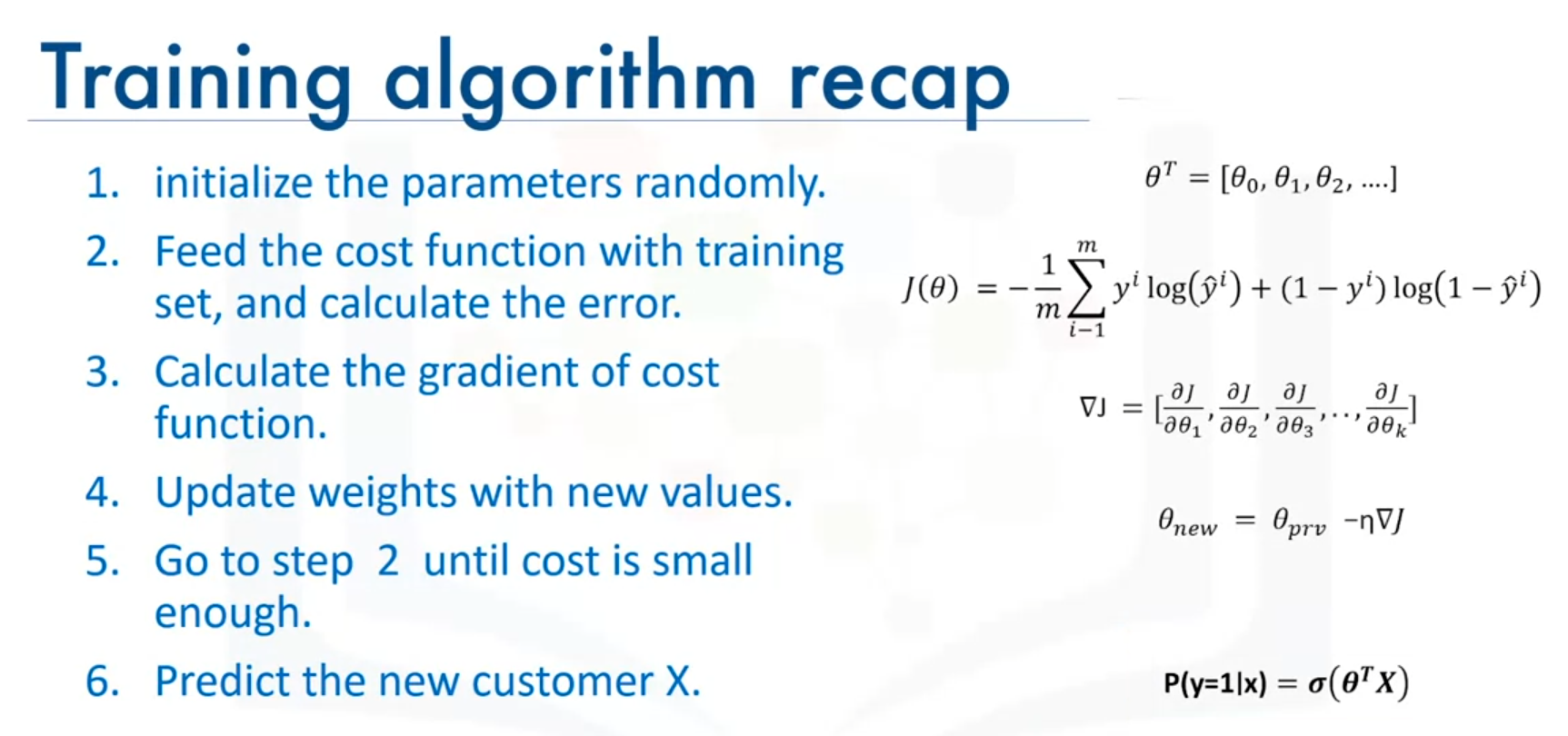
Recap of the Training Process

Initialize Parameters: Set initial random values for the parameters.

Feed Cost Function: Calculate the cost with the current parameters.

Compute Gradient: Find the gradient of the cost function with respect to each parameter.

Update Parameters: Adjust the parameters to move towards minimizing the cost.

Repeat: Continue iterating until the cost is minimized.

Once the parameters are optimized, the model is ready to predict outcomes, such as the probability of a customer churning.

Example Code

import numpy as np

# Sigmoid function
def sigmoid(z):
    return 1 / (1 + np.exp(-z))

# Cost function
def compute_cost(X, y, theta):
    m = len(y)
    h = sigmoid(np.dot(X, theta))
    cost = (-1/m) * np.sum(y * np.log(h) + (1-y) * np.log(1-h))
    return cost

# Gradient descent
def gradient_descent(X, y, theta, learning_rate, iterations):
    m = len(y)
    for i in range(iterations):
        h = sigmoid(np.dot(X, theta))
        theta -= (learning_rate/m) * np.dot(X.T, (h-y))
    return theta

# Example usage
X = np.array([[1, 20], [1, 25], [1, 30]])  # Example feature set
y = np.array([0, 1, 0])                    # Example labels
theta = np.random.rand(2)                  # Initial parameters

learning_rate = 0.01
iterations = 1000

# Train the model
theta = gradient_descent(X, y, theta, learning_rate, iterations)
print("Optimized Parameters:", theta)

This code demonstrates how to implement logistic regression, compute the cost, and perform gradient descent to optimize the model parameters.

Support Vector Machine (SVM)

Introduction to SVM

Support Vector Machine (SVM) is a supervised machine learning algorithm used for classification tasks. It is particularly effective in scenarios where the dataset is not linearly separable. SVM works by finding an optimal separator, known as a hyperplane, that divides the data into different classes.

Example Scenario: Cancer Detection

Imagine a dataset containing characteristics of thousands of human cell samples from patients at risk of developing cancer. Analysis reveals significant differences between benign and malignant samples. SVM can be used to classify new cell samples as either benign or malignant based on these characteristics.

Formal Definition of SVM

A Support Vector Machine is an algorithm that classifies cases by finding a separator. SVM maps the data to a high-dimensional feature space, enabling the separation of data points even when they are not linearly separable in their original space. The separator in this high-dimensional space is a hyperplane.

Non-Linearly Separable Data

In many real-world datasets, such as those with cell characteristics like unit size and clump thickness, the data may be non-linearly separable. This means that a curve, rather than a straight line, is needed to separate the classes. SVM can transform this data into a higher-dimensional space where a hyperplane can be used as a separator.

Kernelling and Kernel Functions

The process of mapping data into a higher-dimensional space is known as kernelling. The mathematical function used for this transformation is called a kernel function. Common types of kernel functions include:

Linear

Polynomial

Radial Basis Function (RBF)

Sigmoid

Each kernel function has its characteristics, advantages, and disadvantages, and the choice of kernel function depends on the dataset.

Optimization: Finding the Best Hyperplane

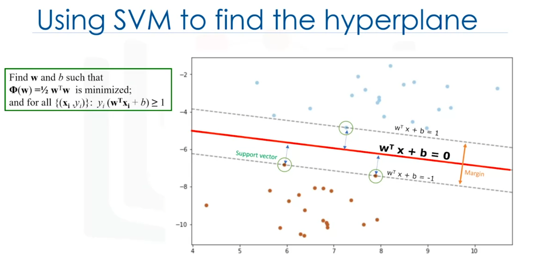
Maximizing the Margin

The goal of SVM is to find the hyperplane that maximizes the margin between the two classes. The margin is the distance between the hyperplane and the nearest data points from each class, known as support vectors.

Support Vectors

Support vectors are the data points that are closest to the hyperplane and are critical in defining the hyperplane. The optimization problem of finding the hyperplane with the maximum margin can be solved using various techniques, including gradient descent.

Equation of the Hyperplane

The hyperplane is represented by an equation involving the parameters $w$ and $b$ . The SVM algorithm outputs the values of $w$ and $b$ , which can then be used to classify new data points. By plugging the input values into the hyperplane equation, the classification can be determined based on whether the result is above or below the hyperplane.

Advantages and Disadvantages of SVM

Advantages

Effective in High-Dimensional Spaces: SVM performs well in datasets with a large number of features.

Memory Efficient: SVM uses a subset of training points (support vectors) in the decision function, which makes it memory efficient.

Disadvantages

Prone to Overfitting: SVM can overfit if the number of features exceeds the number of samples.

Lack of Probability Estimates: SVM does not directly provide probability estimates, which are often desirable in classification tasks.

Computational Inefficiency: SVM is not efficient for very large datasets, especially those with more than 1,000 rows.

Applications of SVM

SVM is widely used in various applications, including:

Image Analysis: Image classification and handwritten digit recognition.

Text Mining: Spam detection, text categorization, and sentiment analysis.

Gene Expression Data Classification: Effective in classifying high-dimensional data.

SVM can also be applied to other machine learning tasks, such as regression, outlier detection, and clustering.

Example: SVM in Python using Scikit-Learn

Here is a code example that demonstrates how to use SVM for a simple classification task in Python using the Scikit-Learn library.

# Import necessary libraries
import numpy as np
import matplotlib.pyplot as plt
from sklearn import datasets
from sklearn.model_selection import train_test_split
from sklearn.svm import SVC
from sklearn.metrics import accuracy_score, classification_report, confusion_matrix

# Load the dataset
iris = datasets.load_iris()
X = iris.data[:, :2]  # We only take the first two features for simplicity
y = iris.target

# Split the data into training and testing sets
X_train, X_test, y_train, y_test = train_test_split(X, y, test_size=0.3, random_state=42)

# Create an SVM model
svm_model = SVC(kernel='linear')  # You can change the kernel to 'rbf', 'poly', etc.

# Train the model
svm_model.fit(X_train, y_train)

# Predict on the test data
y_pred = svm_model.predict(X_test)

# Evaluate the model
print(f"Accuracy: {accuracy_score(y_test, y_pred):.2f}")
print("\nClassification Report:")
print(classification_report(y_test, y_pred))

# Plot decision boundary (for visualization purposes)
def plot_decision_boundary(X, y, model):
    x_min, x_max = X[:, 0].min() - 1, X[:, 0].max() + 1
    y_min, y_max = X[:, 1].min() - 1, X[:, 1].max() + 1
    xx, yy = np.meshgrid(np.arange(x_min, x_max, 0.02),
                         np.arange(y_min, y_max, 0.02))
    Z = model.predict(np.c_[xx.ravel(), yy.ravel()])
    Z = Z.reshape(xx.shape)
    plt.contourf(xx, yy, Z, alpha=0.8)
    plt.scatter(X[:, 0], X[:, 1], c=y, edgecolors='k', marker='o')
    plt.xlabel('Sepal length')
    plt.ylabel('Sepal width')
    plt.title('SVM Decision Boundary')
    plt.show()

# Visualize the decision boundary
plot_decision_boundary(X_test, y_test, svm_model)

Explanation of the Code

Import Libraries: The necessary libraries like NumPy, Matplotlib, and Scikit-Learn are imported.

Load Dataset: The Iris dataset is loaded from Scikit-Learn's built-in datasets. Only the first two features are used to make visualization easier.

Split Dataset: The dataset is split into training and testing sets using train_test_split.

Create and Train SVM Model: An SVM model is created with a linear kernel. The model is then trained using the training data.

Make Predictions: The model makes predictions on the test data.

Evaluate Model: The accuracy, classification report, and confusion matrix are printed to evaluate the model's performance.

Plot Decision Boundary: A function plot_decision_boundary is defined to visualize the decision boundary of the SVM model. The decision boundary is plotted along with the test data points.

Results

Accuracy: The accuracy score indicates how well the SVM model classifies the test data.

Classification Report: Provides detailed performance metrics such as precision, recall, and F1-score for each class.

Decision Boundary Plot: The plot shows how the SVM model separates the different classes based on the two features.

Multiclass Prediction

SoftMax Regression, One-vs-All & One-vs-One for Multi-class Classification

In multi-class classification, data is classified into multiple class labels. Unlike classification trees and nearest neighbors, the concept of multi-class classification for linear classifiers is not as straightforward. Logistic regression can be converted to multi-class classification using multinomial logistic regression or SoftMax regression, a generalization of logistic regression. SoftMax regression is not suitable for Support Vector Machines (SVMs). One-vs-All (One-vs-Rest) and One-vs-One are two other multi-class classification techniques that can convert most two-class classifiers to a multi-class classifier.

SoftMax Regression

SoftMax regression is similar to logistic regression. The SoftMax function converts the actual distances (i.e., dot products) of $x$ with each of the parameters $\theta_i$ for $K$ classes in the range from 0 to $K-1$ . This is converted to probabilities using the following formula:

softmax(x,i) = \frac{e^{-\theta_i^Tx}}{\sum_{j=1}^{K} e^{-\theta_j^Tx}} \quad (1)

The training procedure is almost identical to logistic regression using cross-entropy, but the prediction is different. Consider a three-class example where $y \in {0,1,2}$ (i.e., $y$ can equal 0, 1, or 2). To classify $x$ , the SoftMax function generates a probability of how likely the sample belongs to each class. The prediction is then made using the $argmax$ function:

\hat{y} = argmax_i (softmax(x,i)) \quad (2)

Example

Consider sample $x_1$ . For instance, with real probabilities, the model estimates how likely a sample belongs to each class:

Probability of $\hat{y}=0: softmax(x_1,0)$ = 0.97

Probability of $\hat{y}=1: softmax(x_1, 1)$ = 0.02

Probability of $\hat{y}=2: softmax(x_1,2)$ = 0.01

These probabilities can be represented as a vector, e.g., [0.97, 0.02, 0.01]. To get the class, apply the $argmax$ function, which returns the index of the largest value:

\hat{y} = argmax_i ([0.97, 0.02, 0.01]) = 0

Geometric Interpretation

Each $θ_iTx$ is the equation of a hyperplane, we plot the intersection of the three hyperplanes with 0 in Fig.1 as colored lines, in addition, we can overlay several training samples. We also shade the regions where the value of $θ_iTx$ is largest, this also corresponds to the largest probability. This color corresponds to where a sample $x$ would be classified. For example if the input is in the blue region, the sample would be classified $\hat{y}=0$ , If the input is in the red region it would be classified as $\hat{y}=1$ , and in the yellow region $\hat{y}=2$ . We will use this convention going forward.

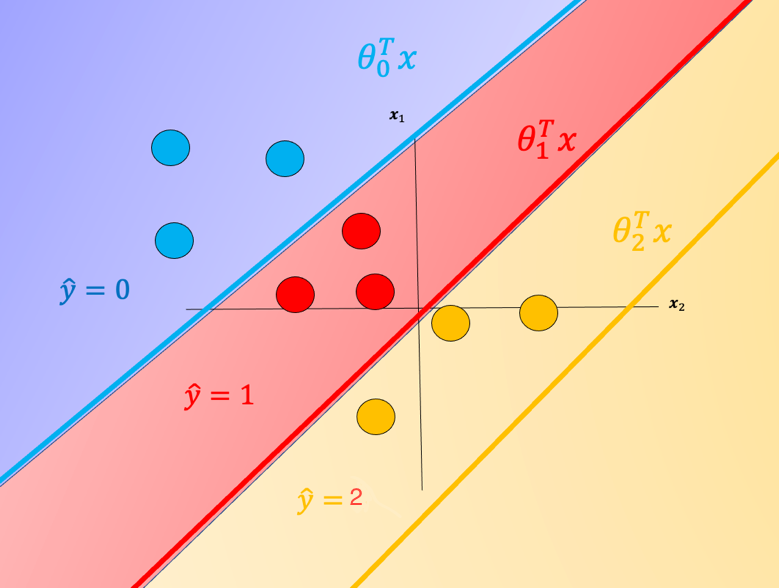
Fig. 1. Equation of a hyperplane. We plot the intersection of the three hyperplanes with 0, in addition we can overlay several samples. We also shade the regions where the value of i is largest.

One problem with SoftMax regression with cross-entropy is it cannot be used for SVM and other types of two-class classifiers.

One vs. All (One-vs-Rest)

For one-vs-All classification, if we have $K$ classes, we use $K$ two-class classifier models, the number of class labels present in the dataset is equal to the number of generated classifiers. First, we create an artificial class we will call this "dummy" class. For each classifier, we split the data into two classes. We take the class samples we would like to classify; the rest of the samples will be labelled as a dummy class. We repeat the process for each class. To make a classification, we can use majority vote or use the classifier with the highest probability, disregarding the probabilities generated for the dummy class.

Although classifiers such as logistic regression and SVM class values are $\{0,1\}$ and $\{−1,1\}$ respectively we will use arbitrary class values. Consider the following samples colored according to class $y=0$ for blue, $y=1$ for red, and $y=2$ for yellow:

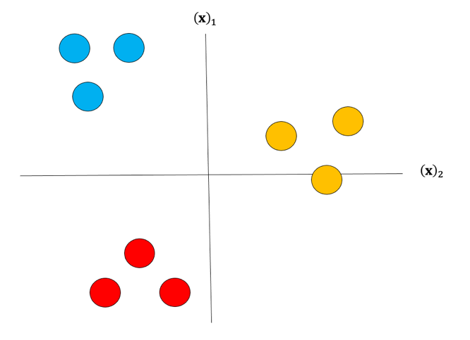
Fig. 2. Samples colored according to class.

For each class we take the class samples we would like to classify, and the rest will be labeled as a “dummy” class. For example, to build a classifier for the blue class we simply assign all other labels that are not in the blue class to the Dummy class, we then train the classifier accordingly. The result is shown in Fig. 3 where the classifier predicts blue $\hat{y}=0$ and in the purple region where we have our “dummy class” $\hat{y}=dummy$ .

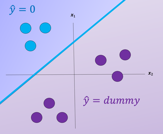
Fig. 3. The classifier predicts blue $\hat{y}=0$ in blue region and dummy class $\hat{y}=dummy$ in purple region.

We repeat the process for each class as shown in Fig. 4, the actual class is shown with the same color and the corresponding dummy class is shown in purple. The color of the space is the actual classifier predictions shown in the same manner as above.

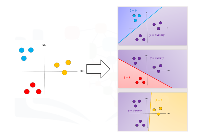
Fig. 4. The classifier predicts $\hat{y}=0,1,2$ in blue, red, and yellow region and dummy class

$\hat{y}=dummy$ in purple region.

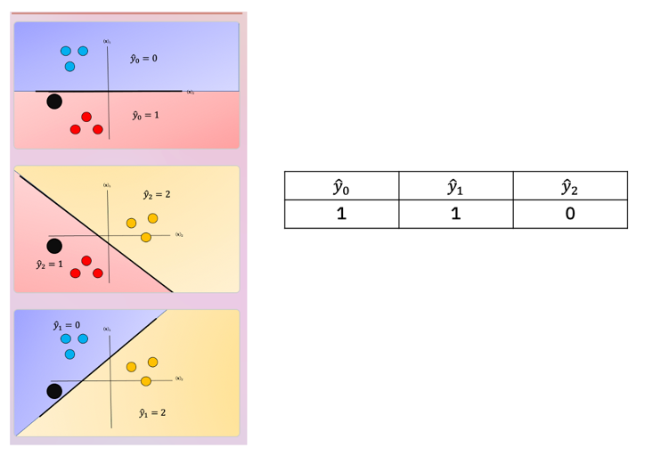
For a sample in the blue region, we would get the following output shown in table 3. You would disregard the dummy classes and select the output $\hat{y}_0=0$ in yellow where the subscript is the classifier number.

Classification Output for a Sample in the Blue Region

Classifier 0:
- Output: $\hat{y}_0 = 0$ (This output is selected)

Classifier 1:
- Output: $\hat{y} = \text{dummy}$ (This classifier is ignored)

Classifier 2:
- Output: $\hat{y} = \text{dummy}$ (This classifier is ignored)

Explanation

For a sample in the blue region, the output for each classifier is evaluated:

Classifier 0 produces a valid output of $\hat{y}_0 = 0$ , which is selected.

Classifier 1 and Classifier 2 both produce dummy outputs, which are disregarded.

As a result, the selected output is $\hat{y}_0 = 0$ , where the subscript indicates the classifier number.

One issue with one vs all is the ambiguous regions as shown in Fig. 5 in purple. In these regions you may get multiple classes for example $\hat{y}_0=0$ and $\hat{y}_1=1$ or all the outputs will equal ”dummy.”

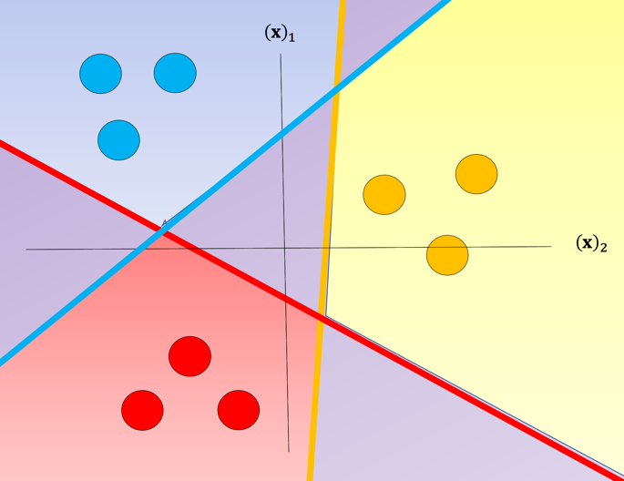
Fig. 5. The classifier predicts all outputs $\hat{y}_0,\hat{y}_1,\hat{y}_2$ will equal "dummy."

There are several ways to reduce this ambiguous region, you can use the output based on the output of the linear function this is called the fusion rule. We can also use the probability of a sample belonging to the actual class as shown in Fig. 6, where we select the class with the largest probability in this case $\hat{y}_0$ ; we disregard the dummy values. These probabilities are scores, as the probabilities are between the dummy class and the actual class not between classes. Just a note packages like Scikit-learn can output probabilities for SVM.

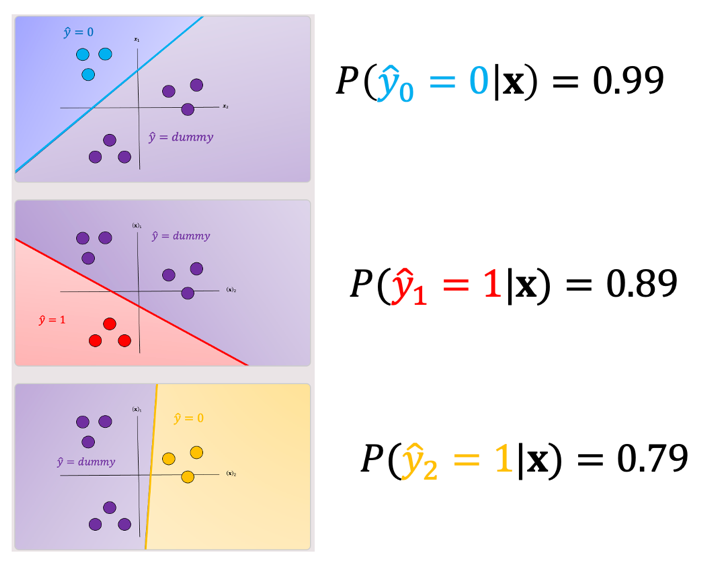
Fig. 6. Probability of a sample belonging to the actual class compared to dummy variable, selects the class with the highest probability.

One-vs-One classification

In One-vs-One classification, we split up the data into each class; we then train a two-class classifier on each pair of classes. For example, if we have class 0,1, and 2, we would train one classifier on the samples that are class 0 and class 1, a second classifier on samples that are of class 0 and class 2, and a final classifier on samples of class 1 and class 2. Fig. 7 is an example of class 0 vs class 1, where we drop training samples of class 2. Using the same convention as above where the color of the training samples are based on their class. The separating plane of the classifier is in black. The color represents the output of the classifier for that particular point in space.

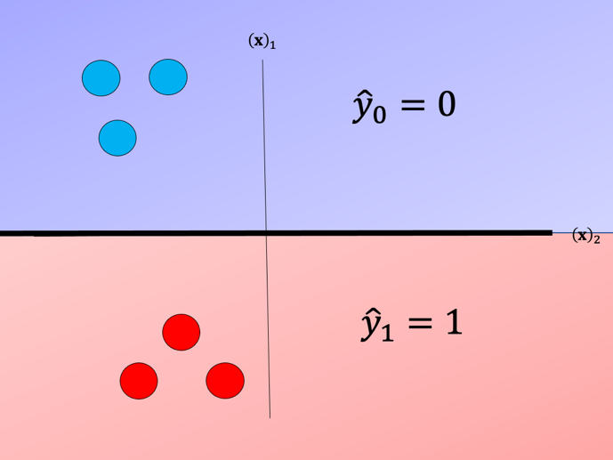
Fig. 7. Probability of a sample belonging to the actual class compared to dummy variable , select the class with the highest probability.

We repeat the process for each pair of classes, in Fig 8. For $K$ classes, we have to train

$K(K−1)/2$ classifiers. So if $K=3$ , we have $(3×2)/2=3$ classes.

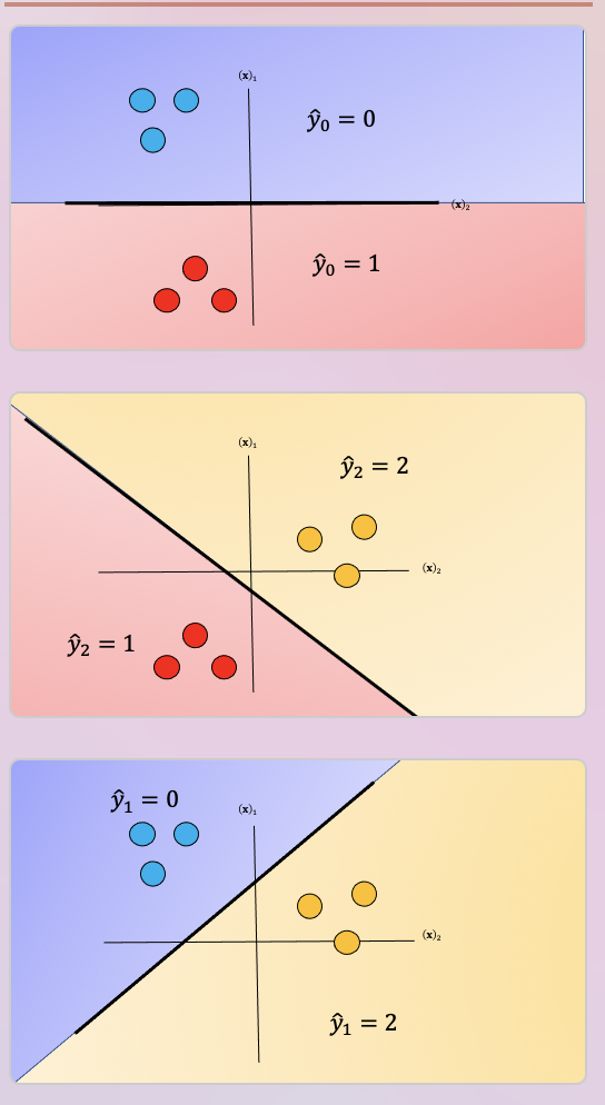
Fig. 8. Probability of a sample belonging to the actual class compared to dummy variable, select the class with the highest probability.

To perform Classification on a sample, we perform a majority vote where we select the class with the most predictions. This is shown in Fig. 9 where the black point represents a new sample and the output of each classifier is shown in the table. In this case, the final output is one as selected by two of the three classifiers. There is also an ambiguous region but it’s smaller, we can also use similar schemes as in One vs all like the fusion rule or using the probability.

GridSearchCV: Hyperparameter Tuning in Machine Learning

Introduction to GridSearchCV

GridSearchCV in Scikit-Learn is a crucial tool for hyperparameter tuning in machine learning. It performs an exhaustive search over specified parameter values for an estimator and systematically evaluates each combination using cross-validation. The goal is to identify the optimal settings that maximize model performance based on a scoring metric such as accuracy or F1-score.

Hyperparameter tuning significantly impacts model performance, preventing underfitting or overfitting. GridSearchCV automates this process, ensuring robust generalization on unseen data, making it an essential tool for data scientists in the machine learning pipeline.

Parameters of GridSearchCV

GridSearchCV has several key parameters:

Estimator: The model or pipeline to be optimized. It can be any Scikit-Learn estimator like LogisticRegression(), SVC(), or RandomForestClassifier().

param_grid: A dictionary or list of dictionaries with parameter names (as strings) as keys and lists of parameter settings to try as values. This allows specifying the hyperparameters for various models to find the optimal combination.

Examples of Hyperparameters for `param_grid`

Logistic Regression:
```
parameters = {'C': [0.01, 0.1, 1],
              'penalty': ['l2'],
              'solver': ['lbfgs']}
```
- C: Inverse of regularization strength; smaller values specify stronger regularization.
- penalty: Specifies the norm of the penalty; 'l2' is ridge regression.
- solver: Algorithm to use in the optimization problem.

Support Vector Machine (SVM):

parameters = {'kernel': ['linear', 'rbf', 'poly', 'sigmoid'],
              'C': np.logspace(-3, 3, 5),
              'gamma': np.logspace(-3, 3, 5)}

kernel: Specifies the kernel type to be used in the algorithm.

C: Regularization parameter.

gamma: Kernel coefficient.

Decision Tree Classifier:
```
parameters = {'criterion': ['gini', 'entropy'],
              'splitter': ['best', 'random'],
              'max_depth': [2*n for n in range(1, 10)],
              'max_features': ['auto', 'sqrt'],
              'min_samples_leaf': [1, 2, 4],
              'min_samples_split': [2, 5, 10]}
```
- criterion: The function to measure the quality of a split.
- splitter: The strategy used to choose the split at each node.
- max_depth: The maximum depth of the tree.
- max_features: The number of features to consider when looking for the best split.
- min_samples_leaf: The minimum number of samples required to be at a leaf node.
- min_samples_split: The minimum number of samples required to split an internal node.

K-Nearest Neighbors (KNN):
```
parameters = {'n_neighbors': [1, 2, 3, 4, 5, 6, 7, 8, 9, 10],
              'algorithm': ['auto', 'ball_tree', 'kd_tree', 'brute'],
              'p': [1, 2]}
```
- n_neighbors: Number of neighbors to use.
- algorithm: Algorithm used to compute the nearest neighbors.
- p: Power parameter for the Minkowski metric.

scoring: A single string or callable to evaluate the predictions on the test set. Common options include accuracy, F1, roc_auc, etc. If none is specified, the estimator's default scorer is used.

n_jobs: The number of jobs to run in parallel. 1 means using all processors.

pre_dispatch: Controls the number of jobs that get dispatched during parallel execution. It can be an integer or expressions like 2*n_jobs, 3*n_jobs, etc., to limit the number of jobs dispatched at once.

refit: If True, refits the best estimator with the entire dataset. The best estimator is stored in the best_estimator_ attribute. Default is True.

cv: Determines the cross-validation splitting strategy. It can be an integer to specify the number of folds, a cross-validation generator, or an iterable. Default is 5-fold cross-validation.

verbose: Controls the verbosity level. Higher values indicate more messages. verbose=0 is silent, verbose=1 shows some messages, and verbose=2 shows more messages.

return_train_score: If False, the cv_results_ attribute will not include training scores. Default is False.

error_score: Value to assign to the score if an error occurs in estimator fitting. np.nan is the default, but it can be set to a specific value.

Applications and Advantages of GridSearchCV

Model Selection: Enables the comparison of multiple models and facilitates the selection of the best-performing one for a given dataset.

Hyperparameter Tuning: Automates the process of finding the optimal hyperparameters, significantly improving model performance.

Pipeline Optimization: Can be applied to complex pipelines involving multiple preprocessing steps and models to optimize the entire workflow.

Cross-Validation: Incorporates cross-validation in the parameter search process, ensuring that the model's performance is robust and not overfitted to a particular train-test split.

Exhaustive Search: Performs an exhaustive search over the specified parameter grid, ensuring the best combination of parameters is found.

Parallel Execution: With the n_jobs parameter, it can leverage multiple processors to speed up the search process.

Automatic Refit: By setting refit=True, GridSearchCV automatically refits the model with the best parameters on the entire dataset, making it ready for use.

Detailed Output: The cv_results_ attribute provides detailed information about the performance of each parameter combination, including training and validation scores, helping to understand the model's behavior.

Practical Example

Below is an example demonstrating the use of GridSearchCV with the Iris dataset to find the optimal hyperparameters for a Support Vector Classifier (SVC).

Import necessary libraries:

import numpy as np
import pandas as pd
from sklearn.datasets import load_iris
from sklearn.model_selection import train_test_split, GridSearchCV
from sklearn.svm import SVC
from sklearn.metrics import classification_report
import warnings
# Ignore warnings
warnings.filterwarnings('ignore')

Load the Iris dataset:
```
iris = load_iris()
X = iris.data
y = iris.target
```
- X: Features of the Iris dataset (sepal length, sepal width, petal length, petal width).
- y: Target labels representing the three species of Iris (setosa, versicolor, virginica).

Split the data into training and test sets:
```
X_train, X_test, y_train, y_test = train_test_split(X, y, test_size=0.2, random_state=42)
```
- test_size=0.2: 20% of the data is used for testing.
- random_state=42: Ensures reproducibility of the random split.

Define the parameter grid:
```
param_grid = {
    'C': [0.1, 1, 10, 100],
    'gamma': [1, 0.1, 0.01, 0.001],
    'kernel': ['linear', 'rbf', 'poly']
}
```
- C: Regularization parameter.
- gamma: Kernel coefficient.
- kernel: Specifies the type of kernel to be used in the algorithm.

Initialize the SVC model:
```
svc = SVC()
```

Initialize GridSearchCV:
```
grid_search = GridSearchCV(estimator=svc, param_grid=param_grid, scoring='accuracy', cv=5, n_jobs=-1, verbose=2)
```
- estimator: The model to optimize (SVC).
- param_grid: The grid of hyperparameters.
- scoring='accuracy': The metric used to evaluate the model's performance.
- cv=5: 5-fold cross-validation.
- n_jobs=-1: Use all available processors.
- verbose=2: Show detailed output during the search.

Fit GridSearchCV to the training data:
```
grid_search.fit(X_train, y_train)
```

Check the best parameters and estimator:

print("Best parameters found: ", grid_search.best_params_)
print("Best estimator: ", grid_search.best_estimator_)

Make predictions with the best estimator:

y_pred = grid_search.best_estimator_.predict(X_test)

Evaluate the performance:
```
print(classification_report(y_test, y_pred))
```
This step outputs a classification report with precision, recall, F1-score, and accuracy.

Output

Best parameters found:  {'C': 1, 'gamma': 0.1, 'kernel': 'rbf'}
Best estimator:  SVC(C=1, gamma=0.1, kernel='rbf')
              precision    recall  f1-score   support

           0       1.00      1.00      1.00        10
           1       1.00      1.00      1.00         9
           2       1.00      1.00      1.00        11

    accuracy                           1.00        30
   macro avg       1.00      1.00      1.00        30
weighted avg       1.00      1.00      1.00        30

Explanation:

The optimal hyperparameters are C=1, gamma=0.1, and kernel='rbf'.

The best estimator with these parameters achieves perfect accuracy (100%) on the test set in this example.

GridSearchCV provides a systematic and automated way to explore hyperparameter space and select the best model configuration, making it an essential tool for improving machine learning models.

Logistic Regression: An Overview

Introduction

1. What is Logistic Regression?

Example:

2. Problems Solved by Logistic Regression

3. Situations to Use Logistic Regression

4. How Logistic Regression Works

Decision Boundary:

Example with a Simple Logistic Regression Model:

5. Formalizing the Problem

Conclusion

Introduction to Linear Regression vs. Logistic Regression

Linear Regression Overview

Python Example: Linear Regression

Challenges with Linear Regression for Classification

Introduction to Logistic Regression

Python Example: Logistic Regression

Key Properties of the Sigmoid Function

Training the Logistic Regression Model

Conclusion

Training a Logistic Regression Model

Objective of Training in Logistic Regression

Example: Customer Churn Prediction

Cost Function in Logistic Regression

Definition

Cost Function for a Single Sample

Mean Squared Error

Optimization: Finding the Best Parameters

Minimizing the Cost Function

Gradient Descent: An Optimization Approach

Steps in Gradient Descent

Gradient Descent Equation

Learning Rate

Recap of the Training Process

Example Code

Support Vector Machine (SVM)

Introduction to SVM

Example Scenario: Cancer Detection

Formal Definition of SVM

Non-Linearly Separable Data

Kernelling and Kernel Functions

Optimization: Finding the Best Hyperplane

Maximizing the Margin

Support Vectors

Equation of the Hyperplane

Advantages and Disadvantages of SVM

Advantages

Disadvantages

Applications of SVM

Example: SVM in Python using Scikit-Learn

Explanation of the Code

Results

Multiclass Prediction

SoftMax Regression, One-vs-All & One-vs-One for Multi-class Classification

SoftMax Regression

Example

Geometric Interpretation

One vs. All (One-vs-Rest)

Classification Output for a Sample in the Blue Region

Explanation

One-vs-One classification

GridSearchCV: Hyperparameter Tuning in Machine Learning

Introduction to GridSearchCV

Parameters of GridSearchCV

Examples of Hyperparameters for param_grid

Applications and Advantages of GridSearchCV

Practical Example

Output

Explanation:

Examples of Hyperparameters for `param_grid`